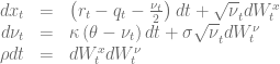
Fokker-Planck Equation, Feller Constraint and Boundary Conditions

May 4, 2013February 19, 2014 hpcquantlibLeave a comment

The Fokker-Planck forward equation is an important tool to calibrate local volatility extensions of stochastic volatility models, e.g. the local vol extension of the Heston model. But the treatment of the boundary conditions – especially at zero instantaneous variance – is notoriously difficult if the Feller constraint

$\sigma^2 \le 2\kappa\theta$

of the square root process for the variance $\nu$

$d\nu_t = \kappa(\theta-\nu_t)dt + \sigma\sqrt{\nu_t}dW$

is violated. The corresponding Fokker-Planck forward equation

$\frac{\partial p}{\partial t} = \frac{\sigma^2}{2}\frac{\partial^2}{\partial \nu^2}(\nu p) - \frac{\partial}{\partial \nu}\left(\kappa\left(\theta-\nu \right ) p\right)$

describes the time evolution of the probability density function p and the boundary at the origin $\nu=0$ is instantaneously attainable if the Feller constraint is violated. In this case the stationary solution [1] of the Fokker-Planck equation

$p_\nu = \frac{\eta^\eta}{\Gamma(\eta)}\frac{\nu^{\eta-1}}{\theta^\eta}e^{-\eta\nu/\theta},\ \eta=\frac{2\kappa\theta}{\sigma^2}$

diverges with

$\lim_{\nu\to 0} p_\nu^{s} \sim \nu^{\eta-1} = \nu^{-\alpha},\ \alpha=1-\frac{2\kappa\theta}{\sigma^2}$

and the zero flow boundary condition at the origin

$\left.\left[ \frac{\sigma^2}{2}\frac{\partial}{\partial \nu} (\nu p) + \kappa(\nu-\theta)p\right]\right|_{\nu=0} = 0$

becomes hard to track numerically. Rewriting the partial differential equation in terms of $q_\nu = v^\alpha p_\nu$ helps to mitigate the problem [2].

$\frac{\partial q}{\partial t} = \nu\frac{\sigma^2}{2}\frac{\partial^2}{\partial \nu^2} q + \kappa(\nu+\theta)\frac{\partial}{\partial \nu}q + \frac{2\kappa^2\theta}{\sigma^2}q$

The corresponding zero flow boundary condition in q reads as follows

$\left.\left[ \nu\frac{\sigma^2}{2}\frac{\partial}{\partial \nu} q + \kappa\nu q\right]\right|_{\nu=0} = 0$

The first step in order to apply the boundary condition is to discretize the transformed Fokker-Planck equation in space direction on a non-uniform grid $\nu_i$

$\frac{\partial q_i}{\partial t} = \alpha_iq_{i-1}+\beta_iq_i+\gamma_iq_{i+1]}$

with

$\begin{array}{rcl} h_i &=& \nu_{i+1}-\nu_i \\ \zeta_i &=& h_{i-1}h_i \\ \zeta^p_i &=& h_i(h_{i-1}+h_i) \\ \zeta^m_i &=& h_{i-1}(h_{i-1}+h_i) \\ \alpha_i &=& \frac{1}{\zeta^m_i}\left(\sigma^2\nu_i-\kappa(\theta+\nu_i)h_i)\right) \\ \beta_i &=& \frac{1}{\zeta_i}\left( -\sigma^2\nu_i+\kappa(\theta+\nu_i)(h_i-h_{i-1}) \right ) +\frac{2\kappa^2\theta}{\sigma^2} \\ \gamma_i &=& \frac{1}{\zeta^p_i}\left( \sigma^2\nu_i + \kappa(\theta+\nu_i)h_{i-1} \right ) \end{array}$

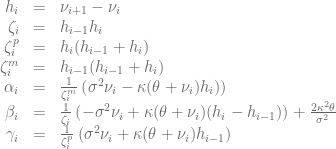
Next step is to discretize the zero flow boundary condition using a second order forward discretization [3] for the derivative $\frac{\partial q}{\partial \nu}$ .

$\left.\left[ \nu\frac{\sigma^2}{2}\frac{\partial}{\partial \nu} q + \kappa\nu q\right]\right|_{\nu=\nu_{i-1}} \approx a_iq_{i-1} + b_iq_{i} + c_iq_{i+1} = 0$

with

$\begin{array}{rcl} \eta_i &=& \frac{1}{h_{i-1}h_i(h_{i-1}+h_i)} \\ a_i &=& - \eta\frac{\sigma^2}{2}\nu_{i-1}\left((h_{i-1}+h_i)^2-h_{i-1}^2 \right ) + \kappa\nu_{i-1} \\ b_i &=& \eta\frac{\sigma^2}{2}v_{i-1}\left(h_{i-1}+h_i \right )^2 \\ c_i &=& -\eta\frac{\sigma^2}{2}v_{i-1} h_{n-1}^2 \end{array}$

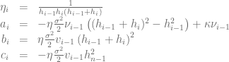
Now the value $q_{0}$ at the boundary $\nu_0$ can be expressed in terms of $q_1$ and $q_2$ .

$q_{0} = \frac{-b_1q_{1} - c_1q_{2}}{a_1}$

This equation can be used to remove the boundary value $q_0$ from the discretization of the transformed Fokker-Planck equation. In the same manner the zero flow boundary condition can be implemented for the upper boundary $\nu_{max}$ and for the original Fokker-Planck equation.

The following parameters of the square-root process will be used to test the different boundary conditions.

$\kappa=2.5,\ \theta=0.2,\ \sigma\in\{0.2, 2.0\}$

The uniform grid $\nu_{min} \le \nu_i \le \nu_{max}$ has 100 or 1000 grid points and the stationary solution $p^s_{\nu_i}$ of the Fokker-Planck equation is chosen as the start configuration on the grid points. The boundaries $v_{min}, v_{max}$ are defined via the inverse cumulated distribution function such that

$\int_0^{v_{min}}p^s_\nu d\nu = \int_{v_{max}}^\infty p_\nu^s d\nu = 1\%$ .

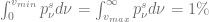
The grid covers 98% of the distribution and this value would not change over time if the boundary conditions are satisfied without discretiszation errors. To test the magnitude of the discretization errors we let the initial solution evolve over one year using 100 time steps with the Crank-Nicolson scheme. The resulting solution 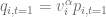$q_{i,t=1} = v_i^\alpha p_{i,t=1}$ is interpolated using cubic splines to get the function $q_\nu$ . The value

$\int_{vmin}^{v_{max}}q_\nu\nu^{-\alpha} d\nu - 98\%$

servers as a quality indicator for the discretization errors of the boundary condition.

As can be seen in the diagram below if $\sigma$ is small then the original Fokker-Planck equation shows smaller discretization errors than the transformed Fokker-Planck equation in $q=v^\alpha p$ . But if $\sigma$ becomes larger and especially if the Feller constraint is violated then the solution of the transformed Fokker-Planck equation clearly outperforms the original solution. As a rule of thumb based on this example one should use the original Fokker-Planck equation if $\frac{2\kappa\theta}{\sigma^2} \ge 2.5$ and the transformed equation otherwise.

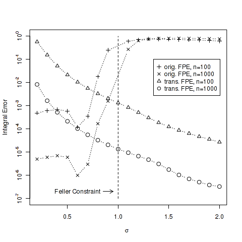
The same techniques can be used to solve the Fokker-Planck equation for the Heston model. The code for the numerical tests is available in the latest QuantLib version from the SVN trunk. The diagram is based on the test FDHestonTest::testSquareRootEvolveWithStationaryDensity.

[1] A. Dragulescu, V. Yakovenko, Probability distribution of returns in the Heston model with stochastic volatility

[2] V. Lucic, Boundary Conditions for Computing Densities in Hybrid Models via PDE Methods

[3] P. Lermusiaux, Numerical Fluid Mechanics, Lecture Note 14, Page 5

Fokker-Planck Forward Equation for the Heston Model

February 10, 2013September 27, 2014 hpcquantlib3 Comments

Consider the stochastic differential equation of the Heston model for the dynamics of the log-spot $x_t = \ln S_t$

$\begin{array}{rcl} dx_t &=& \left(r_t - q_t - \frac{\nu_t}{2}\right)dt + \sqrt\nu_t dW^{x}_t \nonumber \\ d\nu_t&=& \kappa\left(\theta-\nu_t \right ) dt + \sigma\sqrt\nu_t dW^{\nu}_t \nonumber \\ \rho dt &=& dW^{x}_tdW^{\nu}_t \end{array}$

The Fokker-Planck partial differential forward equation describes the time evolution of the probability density function $p(x_t,\nu_t,t)$

$\frac{\partial p}{\partial t} = \frac{1}{2}\frac{\partial^2}{\partial x^2}(\nu p) + \frac{\partial^2}{\partial x \partial \nu} (\rho\sigma\nu p) + \left(\frac{\nu}{2} -r_t+q_t\right)\frac{\partial}{\partial x} p + \frac{\sigma^2}{2}\frac{\partial^2}{\partial \nu^2}(\nu p) - \frac{\partial}{\partial \nu}\left(\kappa\left(\theta-\nu \right ) p\right)$

with the initial condition

$p(x,\nu,t=0) = \delta(x-x_0)\delta(\nu-nu_0)$

where $\delta$ denotes the Dirac delta distribution. A semi-closed form solution for this problem is presented in [1]. When solving the Fokker-Planck forward equation special care must be taken with respect to the boundary conditions, especially if the Feller constraint

$\sigma^2 \le 2\kappa\theta$

is violated. In this case the boundary at the origin $\nu = 0$ is instantaneously attainable. A generalisation of Feller’s zero-flux boundary condition should be applied at the origin [2].

$\left.\left[ \frac{\sigma^2}{2}\frac{\partial}{\partial \nu} (\nu p) + \kappa(\nu-\theta)p + \rho\nu\sigma\frac{\partial p}{\partial x}\right]\right|_{\nu=0} = 0, \ \forall x\in \mathbb{R}^+$

A three point forward differentiation formula can be used to calculate a second order accurate approximation of the partial derivative $\partial_\nu$ for $\nu=0$ [3].

The diagram below shows the solution of the forward equation for the model

$\small{T=1.0, S_0=1,r=0.1, q=0.05, \kappa=2.0, \theta=0.4, \rho=-0.75, v_0=1.2, \sigma=0.4}$

The Feller constraint is violated for $\sigma=2.0$ and this changes the shape of the solution completely.

The code for this example is available here and it is based on the latest QuantLib version from the SVN trunk. It also depends on RInside and Rcpp to generate the plots. In addition the zip contains a short movie clip of the time evolution of the solution for $\sigma=2.0$ .

[1] A. Dragulescu, V. Yakovenko, Probability distribution of returns in the Heston model with stochastic volatility

[2] V. Lucic, Boundary Conditions for Computing Densities in Hybrid Models via PDE Methods

[3] K. A. Kopecky, Numerical Differentiation

Multi-Dimensional Finite Difference Methods on a GPU

December 27, 2012May 4, 2013 hpcquantlib6 Comments

One key aspect for the performance of multi-dimensional finite difference methods based on operator splitting is the performance of the underlying tridiagonal system solver [1]. The authors in [2] have analysed different solver strategies and they have reported a speed-up factor of around 15 between GPU and CPU for the best solver strategy (cyclic reduction) on very large systems. CUDA’s sparse matrix library cuSPARSE contains a routine to solve tridiagonal systems based on cyclic reduction. nVIDIA claims a speed-up factor of around ten compared against Intel’s MKL library [3].

These factors are smaller than the speed-up factors reported for pure Monte-Carlo pricing algorithms. Main reason is that a tridiagonal system solver can not be parallelised by a simple divide and conquer approach like many Monte-Carlo pricing algorithms.

Main classes of the GPU implementation of the Hundsdorfer-Verwer operator splitting scheme are:

GPUFdmLinearOp: implements the FdmLinearOp interface and can be initialized from any instance of FdmLinearOp/FdmLinearOpComposite via the toMatrix()/toMatrixDecomp() methods.
GPUTripleBandLinearOp: GPU based implementation of TripleBandLinearOp. This linear operator can be initialized from any instance of the classes FdmLinearOp/FdmLinearOpComposite via the toMatrix/toMatrixDecomp() methods. The solver for the tridiagonal system is based on cuSPARSE.
GPUHundsdorferScheme: GPU based implementation of the Hundsdorfer-Verwer operator splitting scheme.

The code is available here and it is based on the latest QuantLib version from the trunk, CUDA 4.1 or higher and Cusp 0.3 or higher. As can be seen from the diagrams above the speed-up factor depends on the problem size. Speed-up factors above ten can only be achieved for very large two-dimensional or for medium-sized three-dimensional problems. The GPU precision is defined in cudatypes.hpp by the typedef for the type “real”.

[1] Karel in ’t Hout, ADI finite difference schemes for the Heston model with correlation.

[2] Pablo Quesada-Barriuso, Julián Lamas-Rodríguez, Dora B. Heras, Montserrat Bóo, Francisco Argüello, Selecting the Best Tridiagonal System Solver Projected on Multi-Core CPU and GPU Platforms.

[3] nVIDIA, cuSPARSE

Richardson Extrapolation for American Options

June 10, 2012November 27, 2014 hpcquantlib1 Comment

Popular finite difference schemes like the one-dimensional Crank-Nicholson scheme or multi dimensional operating splitting methods like the Hundsdorfer-Verwer scheme often achieve second order convergence in $\Delta t$ for typical partial differential equations in financial engineering. Unfortunately if these schemes are used together with dynamic programming to price America options the second order convergence is destroyed by the first order convergence of the dynamic programming step.

The Richardson extrapolation is a simple numerical gem to increase the convergence order of a numerical method. Say a numerical method has the following convergence behavior

$f(\Delta t) = f_0 + \alpha \cdot (\Delta t)^n + O((\Delta t)^{n+1})$ .

Please note that this is a more restrictive requirement than to assume that the numerical method is of order n because $\alpha$ does not depend on $\Delta t$ . Now the formula

$R(x, \Delta t) = \frac{x^n f\left(\frac{\Delta t}{x}\right)-f(\Delta t)}{x^n-1} = f_0 + O((\Delta t)^{n+1})$

also has

$\lim_{\Delta t\rightarrow 0} R(x,\Delta t) = f_0$

but the order of convergence of $R(x, \Delta t)$ is n+1. The order does not depend on the particular value of x but often x is chosen to be two. This simple trick can be extended to the case where n is unknown or the Richardson extrapolation can be used m times to increase the order of convergence to n+m [2].

Lets apply the Richardson extrapolation to the pricing of an American Put under the Heston stochastic differential equation. The corresponding partial differential equation

$0 = \frac{\partial u}{\partial t} + \frac{1}{2}S^2v\frac{\partial^2 u}{\partial S^2}+\rho\sigma S\nu \frac{\partial^2 u}{\partial S\partial \nu} + \frac{1}{2}\sigma^2\nu \frac{\partial^2 u}{\partial \nu^2} + rS\frac{\partial u}{\partial S} + \kappa(\theta - \nu)\frac{\partial u}{\partial \nu} -r u$

is solved using the Hundsdorfer-Verwer scheme [1]. The early exercise condition is impressed using dynamic programming after every time step. The parameters of the experiment are

$\small{T=1, K=10, S_0=11, r=0.1, \nu_0=0.0625, \kappa=5, \theta=0.16, \sigma=0.9, \rho=0.1}$ .

As can be seen in the diagram below even though the Richardson extrapolation is a simple formula it increases the convergence by one order from 1.0 to approx. 2.1. If the order is not known a priori then the resulting order is still 1.4.

The source code is available here. It depends on the latest QuantLib version from the SVN trunk.

[1] Karel in ’t Hout, ADI finite difference schemes for the Heston model with correlation.

[2] Eric Hung-Lin Liu, Fundamental Methods of Numerical Extrapolation with Applications.

Accelerate VPP Pricing on the GPU using Preconditioner

January 22, 2012January 30, 2012 hpcquantlibLeave a comment

As outlined in Solving Sparse Linear Systems using CUSP and CUDA a VPP pricing problem can be solved on a GPU using finite difference methods based on the implicit Euler scheme. The matrix inversion is carried out on the GPU using the BiCGStab solver of the numerical library cusp [1]. The optimal exercise problem for the VPP can be solved using dynamic programming for every time slice on the GPU (see [2]).

The lower convergence order in $\Delta t$ of the implicit Euler scheme is not a disadvantage because the hourly optimization step forces $\Delta t = 1h$ anyhow. This step size is small enough for the implicit Euler scheme to obtain a very good accuracy. The explicit Euler scheme is numerically unstable, even if $\Delta t = 1h$ . It converged only for large $\Delta x, \Delta y$ and $\Delta u$ .

Clearly the matrix inversion dominates the overall runtime of the pricing routine. Preconditioning is a standard technique to improve the performance of the involved BiCGStab algorithm. The cusp library supports a set of suited preconditioner for this problem.

Diagonal: preconditioning is very inexpensive to use, but has often limited effectiveness.
Approximate Inverse: Non-symmetric Bridson with different dropping strategies.
Smoothed Aggregation: Algebraic Multi-grid preconditioner based on smoothed aggregation.

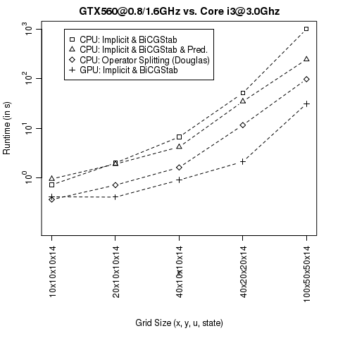
On a CPU QuantLib supports preconditioning based on the Thomas algorithm. This algorithm solves a tridiagonal matrix with $O(8n)$ operations. The corresponding preconditioner can be seen as a natural extension of the diagonal preconditioner. Experiments on a CPU indicate that the tridiagonal preconditioner leads to a significant speed-up for our VPP pricing problem. The upcoming CUSPARSE library of the CUDA 4.1 release contains a tridiagonal solver for the GPU. With the help of a small interface class the CUDA tridiagonal solver can be used as a cusp preconditioner. The source code is available here. The code depends on the latest QuantLib version from the SVN trunk.

The testbed is a VPP contract with $t_{minUp} = t_{minDown} = 2h$ and a maturity of 4 weeks (corresponds to $4*7*24=672$ exercise steps). Therefore in addition to the three dimensions for the stochastic model the problem has a fourth dimension of size $2t_{minUp} + t_{minDown} = 6$ to solve the optimization problem via dynamic programming.

The following diagram shows the different run-times of the algorithms on a GPU and a CPU.

The fastest algorithm on the GPU (implicit Euler scheme with BiCGStab and tridiagonal preconditioner) outperforms the best CPU implementation (operator splitting based on the Douglas scheme) roughly by a factor of ten. The non-symmetric Bridson preconditioner with the dropping strategy from Lin & More on the GPU is the second best algorithm but it ran out of memory on larger grids. The diagonal preconditioner slows down the overall performance on the GPU and the BiCGStab algorithm with the smoothed aggregation preconditioner did not converge.

[1] cusp, Generic Parallel Algorithms for Sparse Matrix and Graph Computations

[2] Pricing of a Virtual Power Plant on a GPU

Bermudan Swaption Pricing based on Finite Difference Methods

December 19, 2011February 18, 2014 hpcquantlibLeave a comment

Even though short rate models like the Hull-White model or the G2++ model are getting a bit long in the tooth these models are still used for risk management or as benchmark models. Since the early days QuantLib supports the pricing of Bermudan swaptions based on trinomial trees. It’s time to compare the performance and accuracy of the trinomial tree pricing algorithm with finite difference methods.

The G2++ model is defined by the following stochastic differential equation

$\begin{array}{rcl} dx_t &=& -ax_tdt+\sigma dW_t^1 \\ dy_t &=& -by_tdt + \eta dW_t^2 \\ dW_t^1 dW_t^2 &=& \rho dt \\ r_t &=& x_t + y_t+\phi_t \\ \phi_t &=& f^M(0,T) +\frac{\sigma^2}{2a^2}\left(1-e^{-aT} \right )^2 + \frac{\eta^2}{2b^2}\left(1-e^{-bT} \right )^2 \\ &+&\rho \frac{\sigma\eta}{ab}\left(1-e^{-aT} \right )\left(1-e^{-bT} \right ) \end{array}$

where $f^M(0,T)$ is denoting the market instantaneous forward rate at time 0 for the maturity T (see. e.g. [1]). The Hull-White model can be seen as a one-dimensional simplification of the G2++ model. The corresponding partial differential equation (PDE) can be derived using the Feynman-Kac theorem.

$\begin{array}{rcl} \frac{\partial V}{\partial t} = ax\frac{\partial V}{\partial x} + by\frac{\partial V}{\partial y} - \frac{\sigma}{2}\frac{\partial^2 V}{\partial x^2} - \frac{\eta}{2}\frac{\partial^2 V}{\partial y^2}-\rho\sigma\eta\frac{\partial^2 V}{\partial x \partial y} + rV \end{array}$

QuantLib supports several operator splitting schemes to solve multi-dimensional PDEs. The SVN trunk contains FDM engines to price Bermudan swaptions under the Hull-White and the G2++ model. Other short rate models like the CIR++ or Black-Karasinski model can be implemented in the same manner.

As can be seen in the diagrams below the finite difference method based pricing engines outperform the trinomial tree based engines.

[1] D. Brigo, F. Mercurio, Interest Rate Models – Theory and Practice

Solving Sparse Linear Systems using CUSP and CUDA

November 13, 2011January 22, 2012 hpcquantlibLeave a comment

A finite difference equation can be represented and solved based on a sparse linear system. When using schemes with implicit parts to solve the equation one needs to calculate the inverse of this sparse matrix. Iterative solvers like the BiCGStab algorithm (plus preconditioner) are tailor-made for these kind of problems. In addition these solvers can easily be adapted to parallel computing architectures like modern GPUs. The cusp library [1] implements a set of common iterative solvers for sparse matrices based on CUDA and thrust [2].

Alternatively operator splitting techniques can be used to solve the problem. In this case only tridiagonal linear systems have to be inverted. The Thomas algorithm (named after Liewellyn Thomas) can solve such systems in $O(n)$ operations instead of $O(n^3)$ operations required by the Gaussian elimination. But it is not easy to parallelize the Thomas algorithm.

On a CPU operator splitting usually outperforms iterative solvers like BiCGStab for the implicit part. The VPP pricing problem from the previous blog entries will now serve as a benchmark to compare the solver performance on the CPU against a GPU. As can be seen in the diagram below on a CPU operator splitting is faster than the BiCGStab solver plus preconditioner. But the BiCGStab on the GPU clearly gains the lead even though the corresponding preconditioner for the GPU has not been implemented yet. Please find the interface class between QuantLib/boost::ublas and cusp here.

[1] cusp, Generic Parallel Algorithms for Sparse Matrix and Graph Computations

[2] thrust, Code at the speed of light

Finite Difference Schemes for the Heston-Hull-White Model

September 11, 2011February 18, 2014 hpcquantlibLeave a comment

The hybrid Heston-Hull-White model is tailor-made to analyse the impact of stochastic interest rates on structured equity notes like e.g. auto-callables.

$\begin{array}{rcl} dS_t &=& (r_t-q_t) S_t dt + \sqrt{v_t} S_t dW_t^S \\ dv_t &=& \kappa_v (\theta_v - v_t) dt + \sigma_v \sqrt{v_t} dW_t^v \\ dr_t & = & \kappa_r(\theta_{r,t}-r_t) dt + \sigma_r dW_t^r \\ \rho_{Sv} dt &=& dW_t^S dW_t^v\\ \rho_{Sr} dt &=& dW_t^S dW_t^r \\ \rho_{vr} dt &=& dW_t^v dW_t^r \end{array}$

Unfortunately a semi-closed solution for european options exists only if at least two correlations are equal to zero which is in general unrealistic. A set of semi-closed approximations for this model can be found here [1]. The QuantLib has a finite difference pricing engine for american, bermudan and european options for the Heston-Hull-White model. This pricing engine supports cash dividends, control variate via the semi-closed Heston Model and pricing different strikes of european options of the same maturity using one backward solver run (especially useful to gain a large speed-up during model calibration.).

The Heston-Hull-White model is a good testbed to test the efficiency of the finite difference schemes based on operator splitting which are implemented in the QuantLib :

Douglas
Craig-Sneyd
Modified Craig-Sneyd
Hundsdorfer-Verwer
Modified Hundsdorfer-Verwer

These operator splitting methods are described here [2]. The testbed contains ten parameter sets of the Heston-Model taken from different publications.

$\begin{array}{|c|c|c|c|c|c|c|c|c|} \hline {\rm Model} & v_0 & \kappa_v & \theta_v & \sigma_v & \rho_{Sv} & r & q & \mbox{Ref} \\ \hline \hline {\rm't\ Hout\ Case\ 1}& 0.04& 1.5& 0.04& 0.3& -0.9& 0.025& 0.0 &[2]\\ {\rm't\ Hout\ Case\ 2} & 0.12& 3.0& 0.12& 0.04& 0.6& 0.01& 0.04 &[2]\\ {\rm't\ Hout\ Case\ 3}& 0.0707&0.6067& 0.0707& 0.2928& -0.7571& 0.03& 0.0 & [2]\\ {\rm't\ Hout\ Case\ 4}& 0.06& 2.5& 0.06& 0.5& -0.1& 0.0507& 0.0469 &[2]\\ {\rm Ikonen\ Toivanen}& 0.0625& 5& 0.16& 0.9& 0.1& 0.1& 0.0 &[3]\\ {\rm Kahl\ J\ddot{a}ckel}& 0.16& 1.0& 0.16& 2.0& -0.8& 0.0& 0.0 &[4]\\ {\rm Equity Case }& 0.07& 2.0& 0.04& 0.55& -0.8& 0.03& 0.035 &\\ {\rm High Correlation}& 0.07& 1.0& 0.04& 0.55& 0.9& 0.02& 0.04& \\ {\rm small\ \sigma_v}& 0.07& 1.0& 0.04& 0.001& -0.75& 0.04& 0.03& \\ \kappa_v=\sigma_v\rho_{Sv}& 0.07& 0.4& 0.04& 0.5& 0.8& 0.03& 0.03 &\\ \hline \end{array}$

The Hull-White parameters are set to $\kappa_r=0.00883$ and $\sigma_r=0.00631$ . The equity interest rate correlation is $\rho_{Sr}=-0.4$ , interest rates and stochastic volatility aren’t correlated $\rho_{vr}=0.$ The benchmark call options have maturity of 5 years, underlying at time $t=0$ is $S_0=100$ and possible strikes are

$K \in \{ 75,85,90,95,100,105,110,115,120,125,130,140,150 \}$ .

The benchmark value is the average relative difference between the reference values and the option prices on the lattice for the different $N_s$ strikes and $N_m$ models.

$\zeta =\frac{1}{N_{s}N_{m}}\sum_{i=1}^{N_{s}N_{m}}\frac{{\rm npv_{ref}^i}-{\rm npv^i}}{K_i}$

The diagram below shows the results of the “Equity Case” for different grid sizes $\{ t, S, v, r\}$ . and with control variate based on the semi–closed Heston Model. Clearly the Douglas scheme is the worst performer, the (modified) Craig-Sneyd and modified Hundsdorfer-Verwer scheme are the winner.

The overall average over the ten models is dominated by the two “pathological” parameter sets “Ikonen-Toivanen” and “Kahl-Jäckel”. Again the Douglas scheme can not compete with the other schemes. The differences between the other schemes are comparable small except for the largest grid where the modified Hundsdorfer-Verwer scheme performs badly.

The relative pricing error with and without control variate is shown in the diagram below for the “Equity Case” Heston model and the modified Craig-Sneyd scheme. On average the usage of the control variate reduces the relative pricing error by a factor of 15.

The source code is available here. It depends on QuantLib 1.1 or higher.If you want to generate the plots you’ll also need R.

[1] L. A. Grzelak, C. W. Oosterleea, Lech A., On the Heston Model with Stochastic Interest Rates.

[2] K.J. in ‘t Hout, S. Foulon, ADI finite difference schemes for option pricing in the Heston model with correlation. Int. J. Numer. Anal. Mod. 7, 303-320 (2010).

[3] S. Ikonen, J. Toivanen, Operator Splitting Methods for American Options with Stochastic Volatility.

[4] C. Kahl, P. Jäckel Not-so-complex logarithms in the Heston model.

VPP Pricing III: Exact Pricing based on Finite Difference Methods

August 7, 2011February 18, 2014 hpcquantlib3 Comments

The total value of a virtual power pant (VPP) can be decomposed in an intrinsic part plus an extrinsic part. The intrinsic value is given by the cash-flows that the VPP would generate based on the current power and gas forward curve. Therefore the intrinsic value can be calculated without defining a stochastic model for the power and gas prices using either linear or dynamic optimization methods. Calculating the extrinsic value implies pricing the VPP exactly to calculate the total value for a given stochastic process. The model in use here is outlined in the article VPP Pricing I: Stochastic Processes & Partial Integro Differential Equation. Exact pricing can be done using least square Monte-Carlo or finite difference methods using dynamic programming for the local optimization [1].

The focus is on the finite difference method, which involves solving the three-dimensional partial integro differential equation

$\begin{array}{rcl} rV&=&\frac{\partial V}{\partial t}+\frac{\sigma_x^2}{2}\frac{\partial^2 V}{\partial x^2}-\alpha x\frac{\partial V}{\partial x}-\beta y \frac{\partial V}{\partial y} \\[6pt]&+&\frac{\sigma_u^2}{2}\frac{\partial^2 V}{\partial u^2}- \kappa u\frac{\partial V}{\partial u} +\rho\sigma_x\sigma_u\frac{\partial^2 V}{\partial x\partial u}\\[6pt] &+&\lambda\int_\mathbb{R}\left(V(x,y+z,u,t)-V(x,y,u,t) \right )\omega(z)dz \\ \end{array}$

An additional fourth dimension is needed to keep track of the different states of the VPP. Based on the characteristics of the VPP type outlined in the article VPP Pricing II: Mixed Integer Linear Programming a VPP with three possible load levels $P \in \{0, P_{min}, P_{max} \}$ has $2 t_{up} + t_{down}$ different states.

Pricing via Monte-Carlo and perfect foresight involves simulating the stochastic process

$\begin{array}{rcl} P_t &=& \exp(p_t + X_t + Y_t) \\ dX_t &=& -\alpha X_tdt + \sigma_x dW_t^x \\ dY_t &=& -\beta Y_{t-}dt+J_tdN_t \\ \omega(J) &=& \eta e^{-\eta J} \\ G_t &=& \exp(g_t + U_t) \\ dU_t &=& -\kappa U_tdt+\sigma_udW_t^u \\ \rho &=& \mathrm{corr} (dW_t^x, dW_t^u) \end{array}$

and optimize the power plant load schedule for each path separately in the same way the intrinsic value is calculated. This procedure will result in an upper bound for the exact price of the VPP. The prices for a 4 weeks VPP contract based on this two methods and with the parameters outlined in VPP Pricing II show almost no differences between the “exact” finite difference method and the perfect foresight upper bound value beside the Monte-Carlo error (s. diagram below, compare with [1]).

The size of the lattice for the finite difference method was

$(t, nPower, nJump, nGas, nStates) = (672, 101, 51, 20, 14)$ .

The code is available here. It depends on the latest QuantLib version from the SVN trunk or the upcoming QuantLib 1.2 release. If you want to generate the plot you’ll also need R

[1] H. van Dijken, D. van Abbena, H.S. Los, C. de Jong, The value of starting up the power plant.

Swing Option: Linear vs. Dynamic Programming II

June 4, 2011May 4, 2013 hpcquantlib4 Comments

In order to get an improved impression on the differences between Monte-Carlo/linear programming and finite difference methods/dynamic programming a more realistic swing option with hourly payoff profile is evaluated based on a German hourly forward curve. The forward curve is taken from the Kyos example download page. The parameterization of the Kluge model is outlined in [1].

With maturity of twelve weeks the example swing option provides $12*7*24=2016$ exercise opportunities. The number of overall exercised swing opportunities is constraint by

$100 \le \sum_{i=1}^{2016} \beta_i \le 500$ .

The size of two dimensions of the finite difference method (dynamic programming) is therefore already been given. 2016 steps are needed in time direction and 500 steps are needed in the “consumed exercises” direction. Together with the two other directions – one for the power price and one dimension for the jump process – and without further simplidsfications this forms a pretty large finite difference problem. The Monte-Carlo based linear programming approach reduces the computational burden but will lead to an upper bound of the swing option price. The diagram below shows the corresponding results.

The code is available here. It depends on the GNU Linear Programming Kit, the Boost Thread library for parallelization and at the time of writing on the latest QuantLib version from the SVN trunk. If you want to generate the plot directly out of the C++ program you also need R, RCPP and RInside. To utilize all CPU cores please use the -DNTHREADS=(number of CPU cores) compiler switch. In addition to run the program you have to download the forward curve German power from the Kyos web page and convert it into a text file EEX_2010-2013.txt of the folliwing format

4-Oct-2010 36.73 32.09 27.32 23.22 25.71 35.60 47.32 …

5-Oct-2010 38.12 31.12 22.76 25.65 27.87 34.60 50.01 …

[1] T. Kluge, Pricing Swing Options and other Electricity Derivatives

HPC-QuantLib

Category: Finite Difference Methods