VPP Pricing IV: Variance Reduction for Perfect Foresight

Even though perfect foresight provides only an upper bound to the real VPP value the differences are often neglectable and the implementation efforts  are small compared with “exact” pricing based on finite difference methods or least square Monte-Carlo. Perfect foresight is the method of choice in conjunction with a linear programming optimizer if the problem contains time-integral constraints. Therefore it is worth to test the efficiency of two standard variance reduction techniques, namely antithetic sampling and quasi Monte-Carlo (QMC) together with a Brownian Bridge. Both methods are explained in [1], antithetic sampling in chapter 4.2 and quasi Monte-Carlo in section 5. Randomized QMC is used to calculate the error estimates for QMC as it is outlined in chapter 5.4.

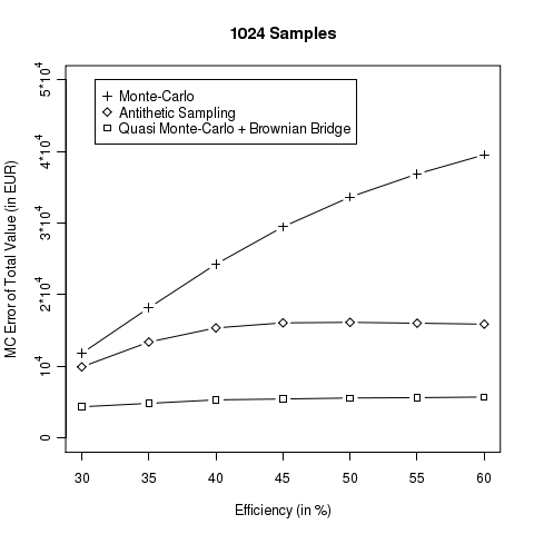
Using the parameterization of the previous section VPP Pricing III, QMC in conjunction with a Brownian Bridge clearly out-performance the other algorithms for a 6 month contract as can be seen in the diagrams below. The code is available here. It depends on the latest QuantLib version from the SVN trunk or the upcoming QuantLib 1.2 release. If you want to generate the plots you’ll also need R.
[1] P. Glasserman, Monte Carlo Methods in Financial Engineering.  ISBN-0387004513

VPP Pricing III: Exact Pricing based on Finite Difference Methods

The total value of a virtual power pant (VPP) can be decomposed in an intrinsic part plus an extrinsic part. The intrinsic value is given by the cash-flows that the VPP would generate based on the current power and gas forward curve. Therefore the intrinsic value can be calculated without defining a stochastic model for the power and gas prices using either linear or dynamic optimization methods. Calculating the extrinsic value implies pricing the VPP exactly to calculate the total value for a given stochastic process. The model in use here is outlined in the article VPP Pricing I: Stochastic Processes & Partial Integro Differential Equation. Exact pricing can  be done using least square Monte-Carlo or finite difference methods using dynamic programming for the local optimization [1].

The focus is on the finite difference method, which involves solving the three-dimensional partial integro differential equation

\begin{array}{rcl} rV&=&\frac{\partial V}{\partial t}+\frac{\sigma_x^2}{2}\frac{\partial^2 V}{\partial x^2}-\alpha x\frac{\partial V}{\partial x}-\beta y \frac{\partial V}{\partial y} \\[6pt]&+&\frac{\sigma_u^2}{2}\frac{\partial^2 V}{\partial u^2}- \kappa u\frac{\partial V}{\partial u} +\rho\sigma_x\sigma_u\frac{\partial^2 V}{\partial x\partial u}\\[6pt] &+&\lambda\int_\mathbb{R}\left(V(x,y+z,u,t)-V(x,y,u,t) \right )\omega(z)dz \\ \end{array}

An additional fourth dimension is needed to keep track of the different states of the VPP. Based on the characteristics of the VPP type outlined in the article VPP Pricing II: Mixed Integer Linear Programming a VPP with three possible load levels P \in \{0, P_{min}, P_{max} \} has 2 t_{up} + t_{down} different states.

Pricing via Monte-Carlo and perfect foresight involves simulating the stochastic process

\begin{array}{rcl} P_t &=& \exp(p_t + X_t + Y_t) \\ dX_t &=& -\alpha X_tdt + \sigma_x dW_t^x \\ dY_t &=& -\beta Y_{t-}dt+J_tdN_t \\ \omega(J) &=& \eta e^{-\eta J} \\ G_t &=& \exp(g_t + U_t) \\ dU_t &=& -\kappa U_tdt+\sigma_udW_t^u \\ \rho &=& \mathrm{corr} (dW_t^x, dW_t^u) \end{array}

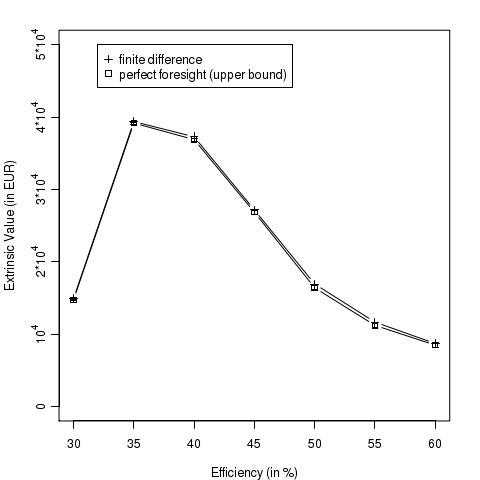
and optimize the power plant load schedule for each path separately in the same way the intrinsic value is calculated. This procedure will result in an upper bound for the exact price of the VPP. The prices for a 4 weeks VPP contract based on this two methods and with the parameters outlined in VPP Pricing II show almost no differences between the “exact” finite difference method and the perfect foresight  upper bound value beside the Monte-Carlo error (s. diagram below, compare with [1]).

The size of the lattice for the finite difference method was

(t, nPower, nJump, nGas, nStates) = (672, 101, 51, 20, 14).

The code is available here. It depends on the latest QuantLib version from the SVN trunk or the upcoming QuantLib 1.2 release. If you want to generate the plot you’ll also need R

[1] H. van Dijken,  D. van Abbena, H.S. Los, C. de Jong, The value of starting up the power plant.