High Performance American Option Pricing

A couple of years ago Andersen, Lake and Offengenden have introduced a new high performance algorithm to price American options for the Black-Scholes-Merton model [1][2]. Basis of the algorithm is an interpolation of the early exercise boundary

$S^\star(t) = B(\tau),\ \tau=T-t$

for a time reversed boundary function $B(\tau)$ with $B(0)=K$ . Knowing the boundary function $B(\tau)$ , the value of an American put option is given by

$\begin{array}{rcl}\displaystyle V(\tau, S)&=& \displaystyle e^{-r\tau}K\Phi\left(-d_-(\tau,S/K)\right)-Se^{-qt}\Phi\left(-d_+(\tau, S/K)\right) \\[5pt] &&\displaystyle + \int_0^\tau r K e^{-r(\tau - u)} \Phi(-d_-(\tau-u, S/B(u) )) du \\[11pt] &&\displaystyle - \int_0^\tau q S e^{-q(\tau - u)} \Phi(-d_+(\tau-u, S/B(u))) du \\[10pt] d_\pm(\tau, x) &=& \displaystyle \frac{\ln{x}+(r-q)\tau \pm\frac{1}{2}\sigma^2\tau}{\sigma\sqrt{\tau}}\end{array}$

and the value of an American call option can be evaluated via the call-put symmetry [3]. The algorithm consists of four separate tasks and the precision of each task is steered by a separate parameter and the choice of an integration algorithm.

The early exercise boundary $B(\tau)$ is interpolated on $n$ Chebyshev nodes [4].
The early exercise boundary $B(\tau)$ is approximated using m fixed point iteration steps. The first iteration is a partial Jacobi-Newton step, the other m-1 steps are ordinary fixed point iterations.
Integrations during the fixed point iterations are either carried out using Gauss-Legendre integration of order l or a tanh-sinh integration with given tolerance ε.
A last integration along the early exercise boundary $B(\tau)$ to get the American option value is using Gauss-Legendre integration of order p or a tanh-sinh integration with given tolerance ν.

It is important for the overall performance that all sub steps lead to a similar accuracy. The parameter space may be best explored with help of a benchmark portfolio, e.g. following [1]

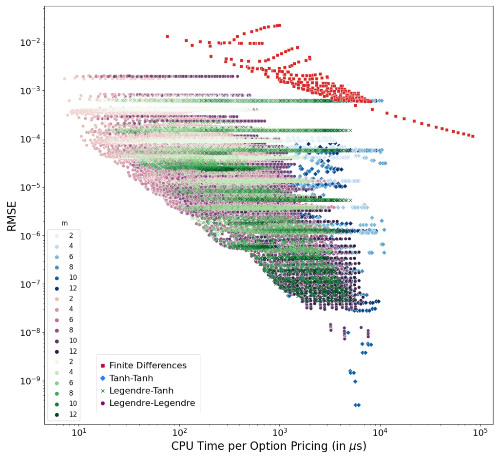
$\begin{array}{rcl} T&\in& \{ 30, 91, 182, 273, 365 \} \\ r &\in& \{2\%, 4\%, 6\%, 8\%, 10\% \} \\ q&\in&\{ 0\%, 4\%, 8\%, 12\%\} \\ S&\in& \{25, 50, 80, 90, 100, 110, 120, 150, 175, 200\} \\ \sigma&\in&\{10\%, 20\%, 40\%, 60\%\}\end{array}$ ,

and the best accuracy per runtime ratios for different parameter configurations. Each dot in the diagram below corresponds to the root mean square error (RMSE) of a different parameter configuration. The RMSE is calculated for all 6000 option prices in the benchmark portfolio and plotted against the runtime of a single option pricing. For comparison the results of the finite difference method have been added but PDEs can not compete with this algorithm (nor can the tree based algorithms in QuantLib).

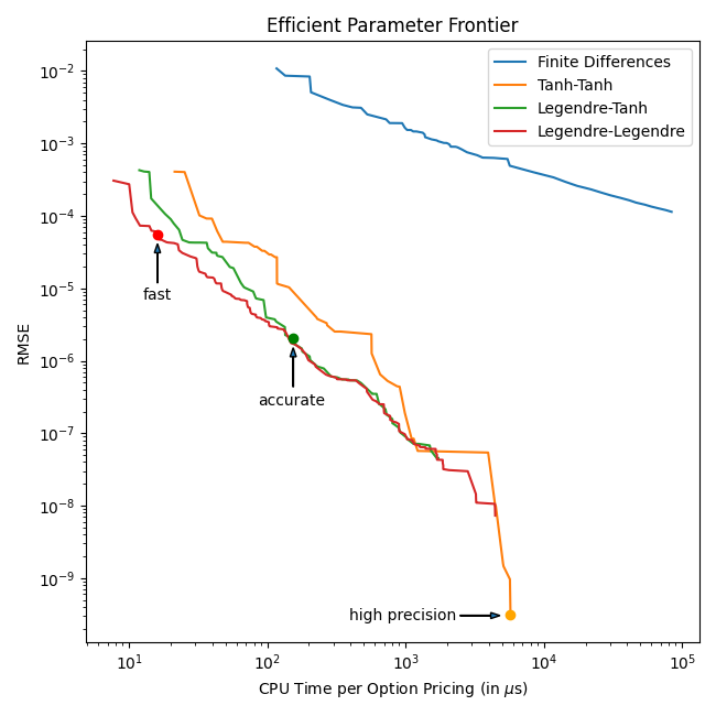
This data set can be used to define the efficient parameter frontiers and take optimal parameter configurations from the frontiers. A fast configuration is Legendre integration for step 3 and 4 and

$(l, n, m, p) = (7,2,7,27)$ ,