January 2019 – HPC-QuantLib

Despite being based on a fairly simple stochastic differential equation

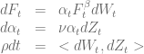
$\begin{array}{rcl} \displaystyle dF_t &=& \alpha_t F_t^\beta dW_t \\ \nonumber d\alpha_t &=& \nu \alpha_t dZ_t \\ \nonumber \rho dt &=& <dW_t, dZ_t> \end{array}$

the corresponding partial differential equation

$\displaystyle \frac{\partial u}{\partial t} - \frac{\nu^2}{2}\frac{\partial u}{\partial x} + \frac{1}{2}e^{2x}F_t^{2\beta}\frac{\partial^2 u}{\partial F^2}+\frac{\nu^2}{2}\frac{\partial^2 u}{\partial x^2}+\rho\nu e^{x_t}F_t^\beta\frac{\partial^2 u}{\partial F \partial x} -ru = 0$

for the SABR model – derived using the variable transformation $x_t = \ln \alpha_t$ together with Ito’s lemma and the Feynman-Kac formula – is quite difficult to solve numerically. Part of the problem is the process of the underlying, which corresponds to a constant elasticity of variance (CEV) model if $\nu$ is zero. This model exhibits a variety of different behaviours depending on the value of $\beta$ and on the boundary conditions. The authors in [1] give a comprehensive overview on this topic. To limit the possible model zoo let’s define

$\displaystyle X\left(F_t\right) = X_t=\frac{F_t^{2(1-\beta)}}{\alpha^2(1-\beta)^2} \ \wedge \ \delta=\frac{1-2\beta}{1-\beta}$

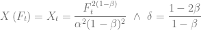
and assume absorbing boundary conditions at $X=0$ if $\delta < 2$ . First step for an implementation of a finite difference scheme is to find efficient limits for the discretization grid. These limits can e.g. be derived from the cumulative distribution function of the underlying process.

$\textrm{Pr}(F \le F_t | F_0) = \begin{cases} 1-{\chi '}^{2}\left( \frac{X_0}{t}; 2-\delta, \frac{X_t}{t}\right), & \textrm{if} \ \delta < 2 \\ \nonumber 1 - {\chi '}^{2}\left( \frac{X_t}{t}; \delta, \frac{X_0}{t}\right), & \textrm{if} \ \delta > 2 \end{cases}$ .

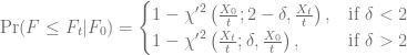
Please notice that the underlying $X(F_t)$ in the first case $\delta < 2$ appears in the non centrality parameter of the non central chi-squared distribution ${\chi '}^{2}$ , hence the calculation of the inverse can only be carried out by a numerical root-finding algorithm. Sankaran’s approximation of the non central chi-squared distribution ${\chi '}^{2}$ can be used to speed-up this method [2]. In the second case $\delta > 2$ the inverse of the equation $\displaystyle \textrm{Pr}(F \le F_t | F_0) = q$ is

$F_t= \left[{t \left({\chi'}^2\right)}^{-1} \left(1-q; \delta, \frac{X_0}{t}\right) \alpha^2(1-\beta)^2\right]^{\frac{1}{2(1-\beta)}}$

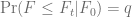
which can be computed using the boost library. In addition adaptive grid refinement around important points and cell averaging around special points of the payoff at maturity [3] improve the accuracy of the CEV finite difference scheme. $F_T$ is only a local martingale when $\delta > 2$ or equivalent $\beta > 1$ . In this case the call-put parity reads [1]

$P_{\delta > 2} = C_{\delta>2} + K - F_0\Gamma\left(-\nu; \frac{X_0}{2t}\right)$

and acts as a litmus test for the implementation of the boundary conditions and the finite difference scheme.

The variance direction $x_t = \ln \alpha_t$ matches a Brownian motion, hence the discretization is straight forward. Operator splitting schemes like Craig-Sneyd or Hundsdorfer-Verwer [4] are tailor made to solve the two dimensional partial differential equation.

The finite difference solver can now be used to compare different approximations with the correct model behaviour and also to compare it with high accurate Monte-Carlo simulations [2]. The model configuration [5]

$F_0=1.0, \alpha=0.35, \beta=0.25, \nu=1.0, \rho=0.25, T=2.0$

should act as a test bed. As can be seen in the diagram below the Monte-Carlo results are in line with the results from finite difference methods within very small error bars. The standard Hagan et al. formula as well as the Le Floc’h-Kennedy [6] log-normal formula deviate significantly from the correct implied volatilities. implvol

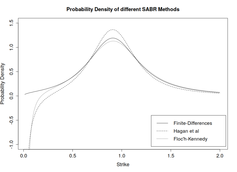
The approximations are not arbitrage free. The probability densities for small strikes turn negative. Hagan’s formula exhibits this behaviour already for larger strikes than the Le Floc’h-Kennedy formula as can be seen in the following diagram. As expected the finite difference solution does not produce negative probabilities.

A note on the Floc’h-Kennedy approximation, the formula becomes numerically unstable around ATM strike levels, hence a second order Taylor expansion is used for moneyness