
A few years ago Andreasen and Huge have introduced an efficient and arbitrage free volatility interpolation method [1] based on a one step finite difference implicit Euler scheme applied to a local volatility parametrization. Probably the most notable use case is the generation of a local volatility surface from a set of option quotes.
Starting point is Dupire’s forward equation for the prices of European call options 


Define the normalized call price 


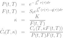
The Dupire forward equation for the normalized prices 

Rewriting this equation in terms of 

The normalized put prices 

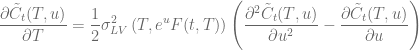
The numerical stability of the original algorithm [1] can be enhanced for deep ITM options by calibrating to calls and puts instantaneously. Also the interpolation scheme has a significant impact on the stability. This topic has been discussed in [2][3]. Using concentrated meshes along the current spot level for the finite difference scheme is of advantage for the stability and accuracy of the algorithm.
In order to stabilize the calculation of the local volatility function

one should evaluate the first order derivative of 

As an example, the diagram below shows different calibrations of the Andreasen-Huge volatility interpolation to a SABR volatility skew at discrete strike sets

for the SABR parameter


The QuantLib implementation is part of the release 1.12.
[1] J. Andreasen, B. Huge, Volatility Interpolation
[2] F. Le Floc’h, Andreasen-Huge interpolation – Don’t stay flat
[3] J. Healy, A spline to fill the gaps with Andreasen-Huge one-step method

Hello,
I’ve finally found a version of andreasen and huge where the dividende and the rate are not equal to zero.
-Do you have a proof for The Dupire forward equation for the normalized prices you get starting from the general Dupire forward equation ?
– I believe in this set up the calibration is going to be made by using the normalized prices you get in the market (which are basically the black scholes normalized prices) ?
– Do you have any other coded implementation other than the one used in quantlib ? I find it hard to get used to that library.
Thank you for the blog.
1. I don’t have my writings any more but you can get from the Dupire equation for normalized prices to the general Dupire forward equation by applying the chain rule many, many times. You might want to check the following paper for more details, esp. formula 15
Click to access Local-Volatility-OpenGamma.pdf
2. Yes.
3. Sorry, no.
Thank you for the response 😉
I am wondering about the following aspect of the Andreasen-Huge method:
once I have computed the option prices for a fixed number of strikes (say 200) using the one-step finite difference solver, how do I get the price for an option with a strike falling in between the 200 discrete strikes?
I am probably just missing something, but this is not clear to me from the paper.
I’d go for either interpolation (If you worry about accuracy you can use many more than 200 steps) or add the needed strikes to the fixed grid in the first place.
I was thinking interpolation, but it doesn’t seem completely trivial. E.g. do you interpolate in price or implied vol? Linear or higher order?
This matters: e.g. consider interpolating linear in price. Then the pdf (prob density) between strikes is zero, so you pdf is a series of delta functions. Quadratic is better, but you still need to figure out how to extrapolate in the high and low wings. Higher order or ivol – how do you know that the interp does not introduce arbitrage?
Making sure all strikes you want are automatically in the original grid would certainly solve the problem, but this is not exactly convenient depending on the application.
Am I making this too complicated?
Sorry, just to add: Andreasen & Huge clealry speak about a continuum of strikes, but as far as I can see they don’t mention how to do the interpolation/extrapolation from the discrete set of strikes at all.
I’ve used spline interpolation in prices. You are right, this will introduce a small arbitrage. W.r.t. extrapolation you can make the price grid large enough such that we do not need to extrapolate.
Thanks for your responses to my questions.
FWIW, it seems to me that a cubic spline ought to have positive convexity throughout since the discrete prices themselves are convex. This interpolation would then correspond to a piecewise constant PDF (since PDF(K) = d2C(K)/dK2), which is guaranteed arb free.
Obviously meant *quadratic* spline, so that d2c(k)/dK2 is constant…