Aim: Develop an exponentially-fitted Gauss-Laguerre quadrature rule to price European options under the Heston model, which outperforms given Gauss-Lobatto, Gauss-Laguerre and other pricing method implementations in QuantLib.
Status quo: Efficient pricing routines for the Heston model
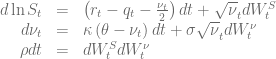
are based on the integration over the normalized characteristic function in the Gatheral formulation

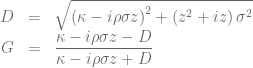
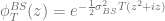
in combination with a Black-Scholes control variate to improve the numerical stability of Lewis’s formula [1][2][3]. The normalized characteristic function of the Black-Scholes model is given by
and the price of a vanilla call option can then be calculated based on
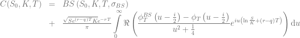
where  is the corresponding Black-Scholes price. Different choices for the volatility of the control variate are discussed in the literature. For the following examples the volatility will be defined by either

or
 .
.
The first one matches the overall variance for  whereas the latter one matches the values of the characteristic functions at the starting point
  of the integration. Usually the latter choice gives better results. Looking at the integrand above one can directly spot a weak point in the algorithm for deep in the money/deep out of the money options. In this case the integrand becomes a highly oscillating function due to the term
 .
.
Second, when using Gauss-Laguerre quadrature the overlap of the weight function  with the characteristic function becomes sub-optimal for very short maturities or small effective volatilities as can be seen with the Black-Scholes characteristic function already.
Third, for very small  the integrand becomes prone to subtractive cancellation errors.
The last issue is easy to overcome by using the second order Taylor expansion of the normalized characteristic for small . The corresponding mathematica script can be seen here.
Rescaling the integrand improves the second issue by rewriting the integral in terms of  with
with
The first problem, the highly oscillating integrand, can be tackled with the exponentially fitted Gauss-Laguerre quadrature rule [4]. The numerical integration of two smooth functions  and
and  with
with

is approximated by a Gauss-Laguerre quadrature rule of the form
 .
.
In this use case the frequency  is
is
 ,
,
and the weights  and nodes
  of the Gauss-Laguerre quadrature rule become functions of the frequency . The algorithm outlined in [4] is too slow to be used at runtime and in the original form only usable up to
  . In order to use it for the Heston model we pre-calculate the weights and nodes for a defined set of frequencies
 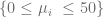 . The closest pre-calculated value
  for a given frequency is then used to evaluate the integral. Of course it would be optimal to use the weights and nodes for instead of but it is far, far better than assuming
  as it is done within the conventional Gauss-Laguerre quadrature rule.
Two techniques are key to get to larger N for the pre-calculated weights and nodes:
- Start the algorithm with to get the standard Gauss-Laguerre weights/nodes and gently increase afterwards. Use the old weights and nodes from the previous up to 20 steps to generate the next starting vector for the Newton solver based on the Lagrange interpolating polynomials.
- Increase “numerical head room” by using the boost multi-precision package instead of double precision. This is only relevant for the pre-calculation. The resulting weights and nodes are stored as normal double precision values.
The source code to generate the weights and nodes for the exponential fitted Gauss-Laguerre quadrature rule is available here.
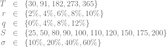
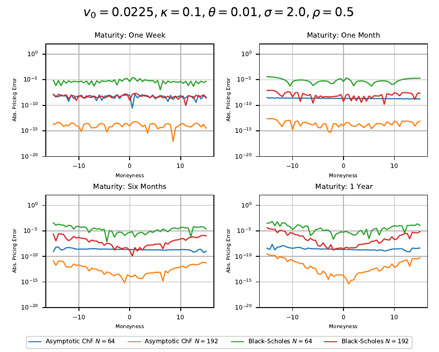
The reference results for the comparison with the other Heston pricing methods are generated using a boost multi-precision version of the Gauss-Laguerre pricing algorithm of order N=2000. Comparison with the results for N=1500 and N=2500 ensures the correctness of the results. The exponentially fitted Gauss-Laguerre quadrature rule is always carried out using N=48 nodes, corresponding to only 48 valuations of the characteristic function. First example model is

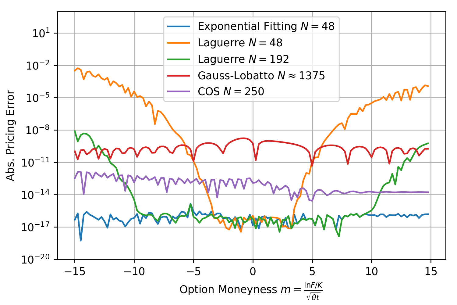
Exponential fitting outperforms the other methods especially when taking the total number of characteristic function valuations into consideration. As expected the method works remarkable well for deep OTM/ITM options and ensures that the absolute pricing error stays below  for an extremely large range of option strikes. Next round, same model but
  .
.
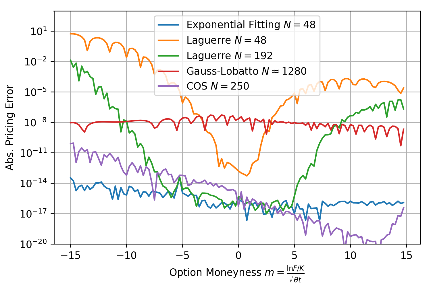
Again the pricing error for exponential fitting stays below  for all moneynesses between -15 and 15 and well below the other methods. Next test, same model but very short maturity with
  . The COS-method with 250 calls of the characteristic function and exponential fitting with N=48 are close together and outperform all other methods.
The same graphs are shown for a variety of different Heston parameters being used in the literature in the following document. The exponentially fitted Gauss-Laguerre quadrature rule with only 64 nodes solves the problem almost always with  for moneynesses between -20 and 20 and maturities between one day and 10 years and outperforms the other methods, especially when taking the number of characteristic function calls needed into consideration. This method can also be extend to larger number of nodes.
The QuantLib implementation of the algorithm is part of the PR#812.
[1] Lewis, A. A simple option formula for general jump-diffusion and other exponential Lévy processes
[2] F. Le Floc’h, Fourier Integration and Stochastic Volatility Calibration.
[3] L. Andersen, and V. Piterbarg, 2010, Interest Rate Modeling, Volume I: Foundations and Vanilla Models, Atlantic Financial Press London.
[4] D. Conte, L. Ixaru, B. Paternoster, G. Santomauro, Exponentially-fitted Gauss–Laguerre quadrature rule for integrals over an unbounded interval.


![\begin{array}{rcl}\displaystyle V(\tau, S)&=& \displaystyle e^{-r\tau}K\Phi\left(-d_-(\tau,S/K)\right)-Se^{-qt}\Phi\left(-d_+(\tau, S/K)\right) \\[5pt] &&\displaystyle + \int_0^\tau r K e^{-r(\tau - u)} \Phi(-d_-(\tau-u, S/B(u) )) du \\[11pt] &&\displaystyle - \int_0^\tau q S e^{-q(\tau - u)} \Phi(-d_+(\tau-u, S/B(u))) du \\[10pt] d_\pm(\tau, x) &=& \displaystyle \frac{\ln{x}+(r-q)\tau \pm\frac{1}{2}\sigma^2\tau}{\sigma\sqrt{\tau}}\end{array}](https://s0.wp.com/latex.php?latex=%5Cbegin%7Barray%7D%7Brcl%7D%5Cdisplaystyle+V%28%5Ctau%2C+S%29%26%3D%26+%5Cdisplaystyle+e%5E%7B-r%5Ctau%7DK%5CPhi%5Cleft%28-d_-%28%5Ctau%2CS%2FK%29%5Cright%29-Se%5E%7B-qt%7D%5CPhi%5Cleft%28-d_%2B%28%5Ctau%2C+S%2FK%29%5Cright%29+%5C%5C%5B5pt%5D+%26%26%5Cdisplaystyle+%2B+%5Cint_0%5E%5Ctau+r+K+e%5E%7B-r%28%5Ctau+-+u%29%7D+%5CPhi%28-d_-%28%5Ctau-u%2C+S%2FB%28u%29+%29%29+du+%5C%5C%5B11pt%5D+%26%26%5Cdisplaystyle+-+%5Cint_0%5E%5Ctau+q+S+e%5E%7B-q%28%5Ctau+-+u%29%7D+%5CPhi%28-d_%2B%28%5Ctau-u%2C+S%2FB%28u%29%29%29+du+%5C%5C%5B10pt%5D+d_%5Cpm%28%5Ctau%2C+x%29+%26%3D%26+%5Cdisplaystyle+%5Cfrac%7B%5Cln%7Bx%7D%2B%28r-q%29%5Ctau+%5Cpm%5Cfrac%7B1%7D%7B2%7D%5Csigma%5E2%5Ctau%7D%7B%5Csigma%5Csqrt%7B%5Ctau%7D%7D%5Cend%7Barray%7D&bg=ffffff&fg=5e5e5e&s=0&c=20201002)
Chebyshev nodes [4].


 ,
,
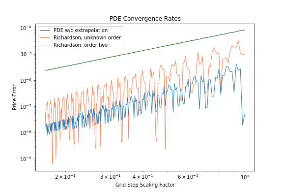
 direction. As expected the order of convergence is increasing from second to fourth order.
 direction is shown below. Finite lattice effects show-up already at relatively small lattices due to the high convergence speed.

 then a lattice size of
 (model definition and further references can be seen
 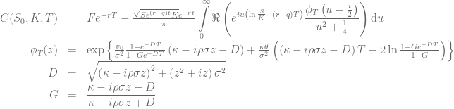 .
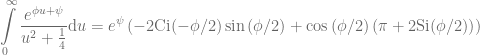
. gives
gives![\phi_T\left(u-\frac{i}{2}\right)\xrightarrow[]{u\rightarrow \infty} e^{\phi u + \psi}](https://s0.wp.com/latex.php?latex=%5Cphi_T%5Cleft%28u-%5Cfrac%7Bi%7D%7B2%7D%5Cright%29%5Cxrightarrow%5B%5D%7Bu%5Crightarrow+%5Cinfty%7D+e%5E%7B%5Cphi+u+%2B+%5Cpsi%7D&bg=ffffff&fg=5e5e5e&s=0&c=20201002)
![\displaystyle \begin{array}{rcl} \phi &=& -\frac{1}{\sigma}\left(v_0 + \kappa\theta T \right)(\sqrt{1-\rho^2} + i\rho)\nonumber \\ \psi &=& \frac{1}{\sigma^2}\left[(\kappa - \rho\sigma/2)(v_0+\kappa\theta T) + \kappa\theta\log\left(4-4\rho^2\right) - i\left(\rho^2\sigma/2- \kappa\rho\right)\frac{v_0+\kappa\theta T}{1-\rho^2} + 2i\kappa\theta\arctan{\frac{\rho}{\sqrt{1-\rho^2}}} \right]\end{array}](https://s0.wp.com/latex.php?latex=%5Cdisplaystyle+%5Cbegin%7Barray%7D%7Brcl%7D+%5Cphi+%26%3D%26+-%5Cfrac%7B1%7D%7B%5Csigma%7D%5Cleft%28v_0+%2B+%5Ckappa%5Ctheta+T+%5Cright%29%28%5Csqrt%7B1-%5Crho%5E2%7D+%2B+i%5Crho%29%5Cnonumber+%5C%5C+%5Cpsi+%26%3D%26+%5Cfrac%7B1%7D%7B%5Csigma%5E2%7D%5Cleft%5B%28%5Ckappa+-+%5Crho%5Csigma%2F2%29%28v_0%2B%5Ckappa%5Ctheta+T%29+%2B+%5Ckappa%5Ctheta%5Clog%5Cleft%284-4%5Crho%5E2%5Cright%29+-+i%5Cleft%28%5Crho%5E2%5Csigma%2F2-+%5Ckappa%5Crho%5Cright%29%5Cfrac%7Bv_0%2B%5Ckappa%5Ctheta+T%7D%7B1-%5Crho%5E2%7D+%2B+2i%5Ckappa%5Ctheta%5Carctan%7B%5Cfrac%7B%5Crho%7D%7B%5Csqrt%7B1-%5Crho%5E2%7D%7D%7D+%5Cright%5D%5Cend%7Barray%7D&bg=ffffff&fg=5e5e5e&s=0&c=20201002)
 and in turn to a very slowly decaying integrand which renders any type of Black-Scholes control variate
 .
.
 .
.
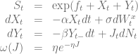
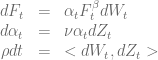
 is a Poisson process with jump intensity
  and
and  is the inverse jump size. To match today’s forward curve
  the function
  is given by


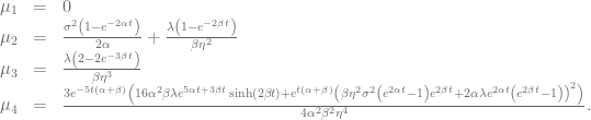
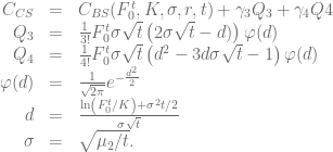
![\displaystyle \mu_n = E\left[\left(Z-E(Z)\right)^n\right] = \sum_{i=0}^n {n\choose i} m_i (-E(Z))^{n-i}](https://s0.wp.com/latex.php?latex=%5Cdisplaystyle+%5Cmu_n+%3D+E%5Cleft%5B%5Cleft%28Z-E%28Z%29%5Cright%29%5En%5Cright%5D+%3D+%5Csum_%7Bi%3D0%7D%5En+%7Bn%5Cchoose+i%7D+m_i+%28-E%28Z%29%29%5E%7Bn-i%7D&bg=ffffff&fg=5e5e5e&s=0&c=20201002)


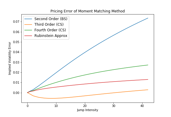 The Corrado/Su fourth order approximation wins only for very small jump intensities, whereas for larger jump intensities the Corrado/Su approximation up to third order competes head-to-head against the Rubinstein formula. Similar picture can be seen for the second test case, few jumps with increasing jump size. For small jumps the fourth order approximation takes the lead but for most of the time the Rubinstein approximation gives the best results.
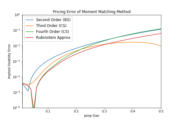

 by utilizing the scaling symmetry of the SABR model [3]
 without lose of generality
 .
. which will be set to
![\displaystyle \alpha \in [0, 1], \ \beta \in [0, 1], \ \nu \in [0, 1]](https://s0.wp.com/latex.php?latex=%5Cdisplaystyle%C2%A0%5Calpha+%5Cin+%5B0%2C+1%5D%2C+%5C+%5Cbeta+%5Cin+%5B0%2C+1%5D%2C+%5C+%5Cnu+%5Cin+%5B0%2C+1%5D&bg=ffffff&fg=5e5e5e&s=0&c=20201002) .
.
 .
.
![\displaystyle \alpha \in [0, 1], \ \beta \in [0, 1], \ \rho \in [-1, 1], \ \nu \in [0, 1], T\in [\frac{1}{12}, 1]](https://s0.wp.com/latex.php?latex=%5Cdisplaystyle%C2%A0%5Calpha+%5Cin+%5B0%2C+1%5D%2C+%5C+%5Cbeta+%5Cin+%5B0%2C+1%5D%2C+%5C+%5Crho+%5Cin+%5B-1%2C+1%5D%2C+%5C+%5Cnu+%5Cin+%5B0%2C+1%5D%2C+T%5Cin+%5B%5Cfrac%7B1%7D%7B12%7D%2C+1%5D&bg=ffffff&fg=5e5e5e&s=0&c=20201002) .
. and
and  quantile of the risk neutral density distribution w.r.t to the ATM volatility of the SABR model. The PDE solver will not only calculate the fair value for
  . Using the scaling symmetry of the SABR model this can be utilized to calculate more prices with new
  and
and  values for
 One could also used gradient tree boosting algorithms like XGBoost or LightGBM. For example the models
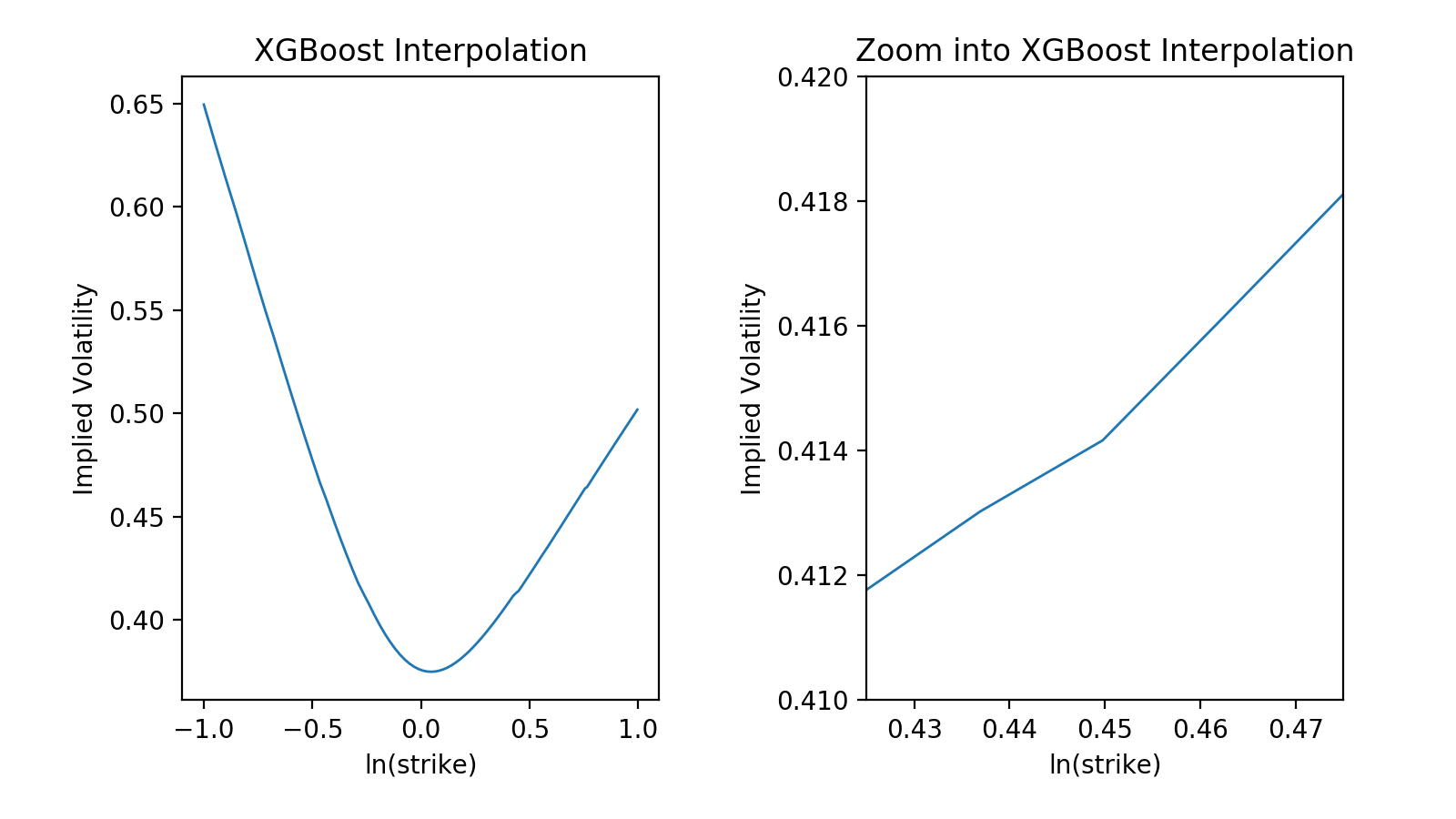 The average run time for the different approximations is shown in the tabular below.
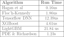

 together with Ito’s lemma and the Feynman-Kac formula – is quite difficult to solve numerically. Part of the problem is the process of the underlying, which corresponds to a constant elasticity of variance (CEV) model if
  and on the boundary conditions. The authors in [1] give a comprehensive overview on this topic. To limit the possible model zoo let’s define
 if
if  . First step for an implementation of a finite difference scheme is to find efficient limits for the discretization grid. These limits can e.g. be derived from the cumulative distribution function of the underlying process.
 .
. in the first case
  , hence the calculation of the inverse can only be carried out by a numerical root-finding algorithm. Sankaran’s approximation of the non central chi-squared distribution
  can be used to speed-up this method [2]. In the second case
  the inverse of the equation
  is
is![F_t= \left[{t \left({\chi'}^2\right)}^{-1} \left(1-q; \delta, \frac{X_0}{t}\right) \alpha^2(1-\beta)^2\right]^{\frac{1}{2(1-\beta)}}](https://s0.wp.com/latex.php?latex=F_t%3D+%5Cleft%5B%7Bt+%5Cleft%28%7B%5Cchi%27%7D%5E2%5Cright%29%7D%5E%7B-1%7D+%5Cleft%281-q%3B+%5Cdelta%2C+%5Cfrac%7BX_0%7D%7Bt%7D%5Cright%29%C2%A0+%5Calpha%5E2%281-%5Cbeta%29%5E2%5Cright%5D%5E%7B%5Cfrac%7B1%7D%7B2%281-%5Cbeta%29%7D%7D&bg=ffffff&fg=5e5e5e&s=0&c=20201002)
 is only a local martingale when
  . In this case the call-put parity reads [1]

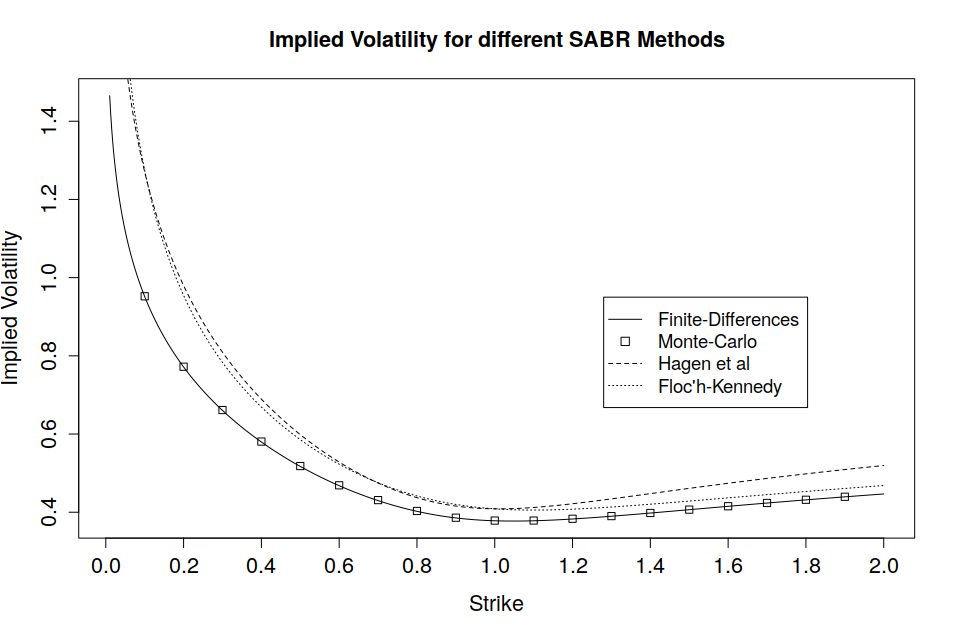
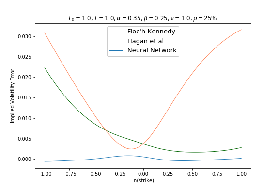
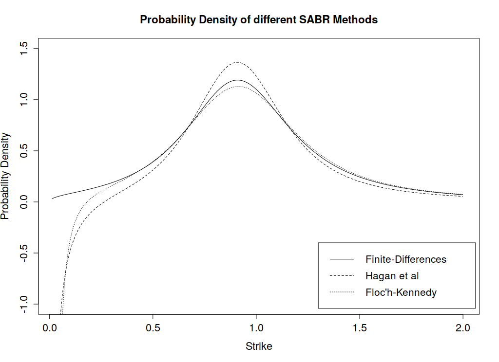 A note on the Floc’h-Kennedy approximation, the formula becomes numerically unstable around ATM strike levels, hence a second order Taylor expansion is used for moneyness
 .
.
