
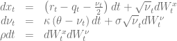
Consider the stochastic differential equation of the Heston model for the dynamics of the log-spot

The Fokker-Planck partial differential forward equation describes the time evolution of the probability density function


with the initial condition

where 

is violated. In this case the boundary at the origin 
![\left.\left[ \frac{\sigma^2}{2}\frac{\partial}{\partial \nu} (\nu p) + \kappa(\nu-\theta)p + \rho\nu\sigma\frac{\partial p}{\partial x}\right]\right|_{\nu=0} = 0, \ \forall x\in \mathbb{R}^+](https://s0.wp.com/latex.php?latex=%5Cleft.%5Cleft%5B+%5Cfrac%7B%5Csigma%5E2%7D%7B2%7D%5Cfrac%7B%5Cpartial%7D%7B%5Cpartial+%5Cnu%7D+%28%5Cnu+p%29+%2B+%5Ckappa%28%5Cnu-%5Ctheta%29p+%2B+%5Crho%5Cnu%5Csigma%5Cfrac%7B%5Cpartial+p%7D%7B%5Cpartial+x%7D%5Cright%5D%5Cright%7C_%7B%5Cnu%3D0%7D+%3D+0%2C+%5C+%5Cforall+x%5Cin+%5Cmathbb%7BR%7D%5E%2B+&bg=ffffff&fg=5e5e5e&s=0&c=20201002)
A three point forward differentiation formula can be used to calculate a second order accurate approximation of the partial derivative 

The diagram below shows the solution of the forward equation for the model


The Feller constraint is violated for 
 The code for this example is available here and it is based on the latest QuantLib version from the SVN trunk. It also depends on RInside and Rcpp to generate the plots. In addition the zip contains a short movie clip of the time evolution of the solution for
[1] A. Dragulescu, V. Yakovenko, Probability distribution of returns in the Heston model with stochastic volatility
[2] V. Lucic, Boundary Conditions for Computing Densities in Hybrid Models via PDE Methods
[3] K. A. Kopecky, Numerical Differentiation

Thanks for your really interesting blog.
I’m trying to understand the zero-flux boundary condition, but I can’t get it.
Can you explain me how do you discretize it?
It will help me a lot
Thanks in advance
Important for the discretization of the boundary condition at \nu=v_{min} is to use forward difference scheme for \partial_\nu p. The easiest forward scheme is the two point formula
\partial_\nu p|_{\nu=v_{min}}=\frac{p_{\nu=v_{min}+\Delta h,x}-p_{\nu=v_{min},x}}{\Delta h}.
If you rewrite the boundary condition using the two point formula then you can get a algebraic equation for p_{\nu=v_{min},x}. This equation can be used at the boundary to eleminate p_{\nu=v_{min},x} from the discretization of the Fokker-Planck equation. Using the three point forward discretization in [3] yields to a better discretization. The following paper gives some example https://cs.uwaterloo.ca/~paforsyt/bc.pdf
This is very intersting work. I have implemented the Heston-type local stochastic volatility model using simple dirichlet boundary condition and I’ trying to develop more general case.
Please tell me any methodology how to reflect this 2-dimensional PDE condition to ADI finite difference scheme?
Repectfully,