February 2013 – HPC-QuantLib

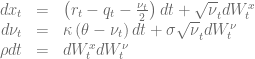
Consider the stochastic differential equation of the Heston model for the dynamics of the log-spot $x_t = \ln S_t$

$\begin{array}{rcl} dx_t &=& \left(r_t - q_t - \frac{\nu_t}{2}\right)dt + \sqrt\nu_t dW^{x}_t \nonumber \\ d\nu_t&=& \kappa\left(\theta-\nu_t \right ) dt + \sigma\sqrt\nu_t dW^{\nu}_t \nonumber \\ \rho dt &=& dW^{x}_tdW^{\nu}_t \end{array}$

The Fokker-Planck partial differential forward equation describes the time evolution of the probability density function $p(x_t,\nu_t,t)$

$\frac{\partial p}{\partial t} = \frac{1}{2}\frac{\partial^2}{\partial x^2}(\nu p) + \frac{\partial^2}{\partial x \partial \nu} (\rho\sigma\nu p) + \left(\frac{\nu}{2} -r_t+q_t\right)\frac{\partial}{\partial x} p + \frac{\sigma^2}{2}\frac{\partial^2}{\partial \nu^2}(\nu p) - \frac{\partial}{\partial \nu}\left(\kappa\left(\theta-\nu \right ) p\right)$

with the initial condition

$p(x,\nu,t=0) = \delta(x-x_0)\delta(\nu-nu_0)$

where $\delta$ denotes the Dirac delta distribution. A semi-closed form solution for this problem is presented in [1]. When solving the Fokker-Planck forward equation special care must be taken with respect to the boundary conditions, especially if the Feller constraint

$\sigma^2 \le 2\kappa\theta$

is violated. In this case the boundary at the origin $\nu = 0$ is instantaneously attainable. A generalisation of Feller’s zero-flux boundary condition should be applied at the origin [2].

$\left.\left[ \frac{\sigma^2}{2}\frac{\partial}{\partial \nu} (\nu p) + \kappa(\nu-\theta)p + \rho\nu\sigma\frac{\partial p}{\partial x}\right]\right|_{\nu=0} = 0, \ \forall x\in \mathbb{R}^+$

A three point forward differentiation formula can be used to calculate a second order accurate approximation of the partial derivative $\partial_\nu$ for $\nu=0$ [3].

The diagram below shows the solution of the forward equation for the model

$\small{T=1.0, S_0=1,r=0.1, q=0.05, \kappa=2.0, \theta=0.4, \rho=-0.75, v_0=1.2, \sigma=0.4}$

The Feller constraint is violated for $\sigma=2.0$ and this changes the shape of the solution completely.

The code for this example is available here and it is based on the latest QuantLib version from the SVN trunk. It also depends on RInside and Rcpp to generate the plots. In addition the zip contains a short movie clip of the time evolution of the solution for $\sigma=2.0$ .

[1] A. Dragulescu, V. Yakovenko, Probability distribution of returns in the Heston model with stochastic volatility

[2] V. Lucic, Boundary Conditions for Computing Densities in Hybrid Models via PDE Methods

[3] K. A. Kopecky, Numerical Differentiation

HPC-QuantLib

Month: February 2013

Fokker-Planck Forward Equation for the Heston Model