February 2014 – HPC-QuantLib

Starting point for a semi-analytical solution of the Fokker-Planck forward equation for the Heston model is the exact sampling algorithm of Broadie and Kaya [1] (for the notation please see [2])

$\begin{array}{rcl} x_t &=& x_0 + m(t) + \sigma(t)Z \nonumber \\ \sigma^2(t) &=& (1-\rho^2)\int_0^t \nu_s ds \nonumber \\ m(t) &=& (r_t-q_t)t - \frac{1}{2}\int_0^t \nu_s ds + \rho\int_0^t \sqrt{\nu_s}dW_s^{(1)} \nonumber \end{array}$

The probability distribution function can be described as

$p(x_t, \nu_t, t) = p(\nu_t, t) p(x_t,t\mid \nu = \nu_t)$

and $p(\nu_t, t)$ is given by a noncentral chi squared distribution. The distribution $p(x_t, t \mid \nu = \nu_t)$ can be calculated using the exact simulation algorithm. In this algorithm the variable $x_t$ is given as a function of two random variables $\int_0^t \nu_s ds$ and $Z$ .

The distribution of $x_t$ can now be derived using the general transformation theorem for random variables: Let X be a random variable with probability density function f. The transformed random variable $Y=h(X)$ has the probability density function

$p(y) = f(h^{-1}(y)) \left| \det \left( \frac{\partial h^{-1}_i(y)}{\partial y_j} \right)\right|$

First step is now to rewrite the exact simulation method in terms of the two random variables

$X_1 = \int_0^t \nu_s ds \ , X_2=Z$ .

The simulation scheme then becomes

$\begin{array}{rcl} x_t &=& x_0+a(t) -\frac{1}{2}X_1 + \frac{\rho\kappa}{\sigma}X_1+\sigma(t) X_2 \nonumber \\\sigma^2(t)&=&(1-\rho^2)X_1 \nonumber \\a(t)&=&(r_t-q_t)t+\frac{\rho}{\sigma}\left( \nu_t-\nu_0-\kappa\theta t \right)\end{array}$

or in terms of the transformed random variable

$\begin{array}{rcl} Y_1 =h_1(X_1,X_2) &=& x_0+a(t)-\frac{1}{2}X_1 + \frac{\rho\kappa}{\sigma}X_1+\sqrt{\left(1-\rho^2\right)X_1}X_2 \nonumber \\ Y_2=h_2(X_1,X_2)&=& X_1 \nonumber\end{array}.$

Let $\phi(x_1)$ be the density function of $X_1$

$\phi(x_1)=\frac{2}{\pi}\int_0^\infty \cos ux_1 \mathrm{Re}(\Phi(u))\mathrm{d}u$

and $X_2$ follows by definition a normal distribution. The joint probability density function of $(X_1, X_2$ ) is then

$f\left( \begin{matrix} x_1 \\ x_2 \end{matrix}\right)=\phi(x_1) \frac{1}{\sqrt{2\pi}}e^{-\frac{x_2^2}{2}}$

with

$\begin{array}{rcl}f\left(h^{-1}(y)\right)&=&f\left(\begin{matrix}y_2 \\ \frac{1}{\sqrt{\left(1-\rho^2\right)y_2}}\left(y_1-x_0-a(t)+\frac{1}{2}y_2-\frac{\rho\kappa}{\sigma}y_2\right)\end{matrix}\right) \nonumber \\ \left|\det \left( \frac{\partial h^{-1}_i(y)}{\partial y_j} \right)\right| &=& \frac{1}{\sqrt{\left(1-\rho^2\right)y_2}} \end{array}.$

This yields to the semi-analytical formula for the solution of the Fokker-Planck equation because by definition $p(x_t,t \mid \nu = \nu_t)$ is the distribution density function of $Y_1$ , which is given by

$p(x_t,t \mid \nu = \nu_t) = \int_0^\infty \mathrm{d}y_2 p(y_1, y_2)\mid_{y_1=x_t} = \int_0^\infty \mathrm{d}y_2 \left[f\left(h^{-1}(y)\right)\left|\det \left( \frac{\partial h^{-1}_i(y)}{\partial y_j} \right)\right| \right]_{y_1=x_t}$

The integration over $y_2$ can be carried out using e.g. the Simpson integral rule together with the Cornish-Fisher expansion, which gives an upper bound for the truncation of the upper limit of the integration.

The contour plots below show the probability density function of the Heston model for some example parametrisations.

$\begin{array}{|c|c|c|c|c|c|c|c|c|} \hline {\rm Parameters} & x_0 & \nu_0 & r & q & \kappa & \theta & \sigma & \rho \\ \hline \hline a & 4.6052 & 0.4 & 5\% & 2.5\% & 1.0 & 0.4 & 0.8 & -75\% \\ \hline b & 4.6052 & 0.4 & 5\% & 2.5\% & 1.0 & 0.4 & 0.8 & \ \ 75\% \\ \hline c & 4.6052 & 0.4 & 5\% & 2.5\% & 1.0 & 0.4 & 0.4 & -75\% \\ \hline d & 4.6052 & 0.4 & 5\% & 2.5\% & 1.0 & 0.4 & 0.4 & \ \ \ \ 0\% \\ \hline \end{array}$

The example code is available here and depends on the upcoming QuantLib version 1.4.

[1] M. Broadie, Ö. Kaya, Exact Simulation of Stochastic Volatility and other Affine Jump Diffusion Processes

[2] K. Spanderen, Probability Distribution of the Heston Model, Part I

[3] R.U. Seydel, Tools for Computational Finance, pp 86

The Heston model is defined by the following stochastic differential equation of the log spot $x_t = \ln S_t$

$\begin{array}{rcl} dx_t &=& \left(r_t - q_t - \frac{\nu_t}{2}\right)dt + \sqrt\nu_t dW^{x}_t \nonumber \\ d\nu_t&=& \kappa\left(\theta-\nu_t \right ) dt + \sigma\sqrt\nu_t dW^{\nu}_t \nonumber \\ \rho dt &=& dW^{x}_tdW^{\nu}_t \end{array}$

To a significant extent the popularity of the Heston model is based on the fact that semi-closed formulas for vanilla European options exist using the characteristic function of the model. The time evolution of the probability density function $p(x_t, v_t, t)$ is given by the corresponding Fokker-Planck equation [1]

$\frac{\partial p}{\partial t} = \frac{1}{2}\frac{\partial^2}{\partial x^2}(\nu p) + \frac{\partial^2}{\partial x \partial \nu} (\rho\sigma\nu p) + \left(\frac{\nu}{2} -r_t+q_t\right)\frac{\partial}{\partial x} p + \frac{\sigma^2}{2}\frac{\partial^2}{\partial \nu^2}(\nu p) - \frac{\partial}{\partial \nu}\left(\kappa\left(\theta-\nu \right ) p\right)$

with the initial condition

$p(x,\nu,t=0) = \delta(x-x_0)\delta(\nu-\nu_0)$

The reduced probability density function

$p(x_t, t \mid x_0,\nu_0) = \int_0^\infty p(x_t, \nu_t, t) d\nu$

for this initial value problem can be calculated using a semi-closed integral formula [2]

$\begin{array}{rcl} \Gamma &=& \kappa+i\rho\sigma p_x \\ \Omega &=& \sqrt{\Gamma^2 + \sigma^2\left(p_x^2-ip_x \right )} \\ p(x_t, t \mid \nu_0) &=& \int_{-\infty}^\infty \frac{dp_x}{2\pi}\exp\left( ip_x (x_t-x_0 -(r-q)t) -\nu_0 \frac{p_x^2-ip_x}{\Gamma + \Omega \coth\left(\Omega t/2 \right )} \right) \\ && \ \ \ \ \ \ \ \ \times \exp\left(-\frac{2\theta\kappa}{\sigma^2}\ln\left(\cosh\frac{\Omega t}{2} + \frac{\Gamma}{\Omega} \sinh \frac{\Omega t}{2}\right )+\frac{\kappa\Gamma\theta t}{\sigma^2} \right) \\ &=& \int_{-\infty}^\infty \frac{dp_x}{2\pi} \tilde{p}(p_x,t \mid \nu_0) \end{array}$

This gives the opportunity to write a pricing engine for arbitrary European payoffs. The value of an European option with payoff function $P(S_t) \in \mathbb{L}^2$ at maturity $t$ is given by

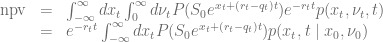
$\begin{array}{rcl} \text{npv} &=& \int_{-\infty}^\infty dx_t\int_{0}^\infty d\nu_t P(S_0 e^{x_t+(r_t-q_t)t})e^{-r_t t} p(x_t,\nu_t,t) \\ &=& e^{-r_t t}\int_{-\infty}^\infty dx_t P(S_0 e^{x_t+(r_t-q_t)t})p(x_t,t \mid x_0,\nu_0) \end{array}$

The calculation needs two nested integrations which can be carried out efficiently using e. g. the Gauss-Lobatto algorithm. The solution of the equation

$| \tilde{p}(p_x, t \mid \nu_0)| = \text{QL\_EPSILON}$

determines the upper boundary for the integration over $p_x$ . The boundaries $\left[ -x_{min}, x_{max}\right]$ for the integration over $x_t$ are chosen such that the interval covers ten times the expected variance

$-x_{min} = x_{max}=10\sqrt{\int_0^{t}E\left[ \nu_t \right ] dt} = 10\sqrt{\theta t + \frac{1}{\kappa}\left(\nu_0-\theta\right)\left(1-e^{-\kappa t}\right)}$

Obviously the nested integration makes this algorithm more tricky than the standard ways to price plain vanilla European options but it is not limited to vanilla payoffs. The implementation of this algorithm can be found here within the QuantLib trunk on Github.

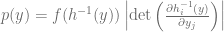
Broadie and Kaya [1] have outlined an algorithm to sample from the full probability density function $p(x_t, \nu_t, t \mid x_0, \nu_0)$ instead of the reduced density function $p(x_t, t \mid x_0, \nu_0)$ . Starting point for this algorithm is the exact solution of the Heston stochastic differential equation

$\begin{array}{rcl} x_t &=& x_o + (r_t-q_t)t - \frac{1}{2}\int_0^t \nu_s ds + \rho\int_0^t \sqrt{\nu_s} dW_s^{(1)} + \sqrt{1-\rho^2}\int_0^t \sqrt{\nu_s} dW_s^{(2)} \nonumber \\ \nu_t &=& \nu_0 + \kappa\theta t - \kappa \int_0^t \nu_s ds + \sigma \int_0^t\sqrt{\nu_s}dW_s^{(1)} \nonumber \end{array}$

The probability density function of the variance process $\nu_t$ is given by a noncentral chi-squared distribution

$\nu_t = \frac{\sigma^2\left( 1-e^{-\kappa t}\right)}{4\kappa}\chi_d^{'2}\left(\frac{4\kappa e^{-\kappa t}}{\sigma^2\left(1-e^{-\kappa t}\right)}\nu_0\right), d=\frac{4\theta\kappa}{\sigma^2}$

The distribution $\Psi(0,t)$ of the integral $\int_0^t \nu_s ds$ conditional on $\nu_t$ and $\nu_0$ can be calculated via the characteristic function

$\begin{array}{rcl} \text{Pr}(\Psi(t) \le x)&=& \frac{2}{\pi}\int_0^\infty \frac{\sin ux}{u}\text{Re}(\Phi(u)) du \\ \\ \Phi(a)&=& \frac{\gamma(a)e^{-\frac{1}{2}(\gamma(a)-\kappa)t} \left(1-e^{-\kappa t}\right)} {\kappa\left(1-e^{\gamma(a)t}\right)} \exp\left( \frac{\nu_t+\nu_0}{\sigma^2} \left[ \frac{\kappa\left(1+e^{-\kappa t}\right)}{1-e^{-\kappa t}} - \frac{\gamma(a)\left(1+e^{-\gamma(a)t}\right)}{1-e^{-\gamma(a)t}} \right] \right) \\ && \times \frac{I_{0.5d-1} \left( \sqrt{\nu_0\nu_t} \frac{4\gamma (a) e^{-0.5\gamma(a)t}}{\sigma^2\left(1-e^{-\gamma(a)t}\right)}\right)}{ I_{0.5d-1} \left( \sqrt{\nu_0\nu_t} \frac{4\kappa e^{-0.5\kappa t}}{\sigma^2\left(1-e^{-\kappa t}\right)}\right)} \\ && \times \frac{\exp\left((0.5d-1) \left[-\frac{1}{2}\gamma(a)t + \ln \frac{\gamma(a)}{1-e^{-\gamma(a)t}} \right]\right)}{\left(\frac{\gamma(a) e^{-0.5\gamma(a)t} }{ 1-e^{-\gamma(a)t}}\right)^{0.5d-1}} \\ \\ \gamma(a)&=&\sqrt{\kappa^2-2 i \sigma^2 a} \end{array}$

The modified Bessel function of first kind $I_{0.5d-1}(z)$ can be evaluated using series expansion for small and medium $|z|$ or asymptotic approximation for large $|z|$ [5]. Unfortunately Boost provides only real versions of the Bessel functions and the copyright status of older complex valued Fortran77 routine is vague. Therefore QuantLib comes with its own implementation.

Please notice that $\Phi(a)$ is already a continuous version of the characteristic function and therefore the integration does not need to track the branches of $arg(z)$ when calculating the complex valued Bessel function [4].

The integration over the characteristic function is best done using either Gauss-Laguerre, Gauss-Lobatto or trapezoidal rule. The two later algorithms need to truncate the integration at some upper bound. First guess for a truncation limit can be taken from the Cornish-Fisher expansion for some very small $\epsilon$ . The moment-generating function $\Phi(a)$ can be used to get the first, second and third moment of the distribution via finite difference quotient.

$m_n = E(X^n) = \frac{d^n}{dy^n}\Phi(x+iy)\Big|_{x=y=0}$

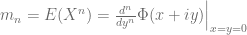
The next term is now fairly easy to calculate

$\int_0^t \sqrt{\nu_s} dW_s^{(1)} = \frac{1}{\sigma}\left( \nu_t - \nu_0 - \kappa\theta t+\kappa \int_0^t \nu_s ds \right)$

The log spot process can now be sampled using a standard normal random variable $Z$ and

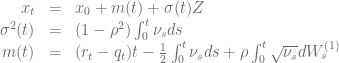
This sampling algorithm is exact even for very large time steps and therefore gives some advantages for quasi random Monte-Carlo methods but the inversion of the integration of the characteristic function is also very slow. The algorithm is implemented within the HestonProcess class.

[1] I. Clark, Foreign Exchange Option Pricing: A Practitioners Guide, p. 113

[2] A. Dragulescu, V. Yakovenko, Probability distribution of returns in the Heston model with stochastic volatility

[3] M. Broadie, Ö. Kaya, Exact Simulation of Stochastic Volatility and other Affine Jump Diffusion Processes

[4] R. Lord, Efficient pricing algorithms for exotic derivatives, p. 40

[5] J.R. Culham, Bessel Functions of the First and Second Kind