In a recent paper [1] Lech Grzelak has introduced his Collocating Local Volatility Model (CLV). This model utilises the so called collocation method [2] to map the cumulative distribution function of an arbitrary kernel process onto the true cumulative distribution function (CDF) extracted from option market quotes.
Starting point for the collocating local volatility model is the market implied CDF of an underlying  at time
  :
:

The prices can also be given by another calibrated pricing model, e.g. the Heston model or the SABR model. To increase numerical stability it is best to use OTM calls and puts.
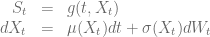
The dynamics of the spot process should be given by some stochastic process  and a deterministic mapping function
  such that

The mapping function ensures that the terminal distribution of given by the CLV model matches the market implied CDF. The model then reads
The choice of the stochastic process does not influence the model prices of vanilla European options – they are given by the market implied terminal CDF – but influences the dynamics of the forward volatility skew generated by the model and therefore the prices of more exotic options. It is also preferable to choose an analytical trackable process to reduce the computational efforts.
The collocation methods outlined in [2] defines an efficient algorithm to approximate the mapping function based on a set of collocation points  for a given set of maturities
  and
and  interpolation points per maturity
  . Let
. Let  be the market implied CDF for a given expiry . Then we get
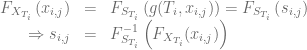
for the collocation points with  .
.
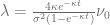
The optimal collocation points are given by the abscissas of the Gaussian quadrature for the terminal distribution of  . The simplest choice is a normally distribute kernel process like the Ornstein-Uhlenbeck process
 .
.
The corresponding collocation points of the Normal-CLV model are then given by
![\begin{array}{rcl} x_j(t) &=& \mathbb{E}\left[X_t\right] + \sqrt{\mathbb{V}ar\left[X_t\right]} x_j^{\mathcal{N}(0,1)} \nonumber \\ &=& \theta + \left(X_0 - \theta)e^{-\kappa t}\right) + \sqrt{\frac{\sigma^2}{2\kappa}\left(1-e^{-2\kappa t}\right)} x_j^{\mathcal{N}(0,1)}, \ j=1,...,n\end{array}](https://s0.wp.com/latex.php?latex=%5Cbegin%7Barray%7D%7Brcl%7D+x_j%28t%29+%26%3D%26+%5Cmathbb%7BE%7D%5Cleft%5BX_t%5Cright%5D+%2B+%5Csqrt%7B%5Cmathbb%7BV%7Dar%5Cleft%5BX_t%5Cright%5D%7D+x_j%5E%7B%5Cmathcal%7BN%7D%280%2C1%29%7D%C2%A0+%5Cnonumber+%5C%5C+%26%3D%26+%5Ctheta+%2B+%5Cleft%28X_0+-+%5Ctheta%29e%5E%7B-%5Ckappa+t%7D%5Cright%29+%2B+%5Csqrt%7B%5Cfrac%7B%5Csigma%5E2%7D%7B2%5Ckappa%7D%5Cleft%281-e%5E%7B-2%5Ckappa+t%7D%5Cright%29%7D+x_j%5E%7B%5Cmathcal%7BN%7D%280%2C1%29%7D%2C+%5C+j%3D1%2C...%2Cn%5Cend%7Barray%7D&bg=ffffff&fg=5e5e5e&s=0&c=20201002)
in which the collocation points  of the standard normal distribution can be calculated by QuantLib’s Gauss-Hermite quadrature implementation
Array abscissas = std::sqrt(2)*GaussHermiteIntegration(n).x()
Lagrange polynomials [3] are an efficient interpolation scheme to interpolate the mapping function between the collocation points

Strictly speaking Lagrange polynomials do not preserve monotonicity and one could also use monotonic interpolation schemes supported by QuantLib’s spline interpolation routines. As outlined in [2] this method can also be used to approximate the inverse CDF of an “expensive” distributions.
Calibration of the Normal-CLV model to market prices is therefore pretty fast and straight forward as it takes the calibration of  .
.
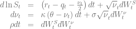
Monte-Carlo pricing means simulating the trackable process and evaluate the Lagrange polynomial if the value of the spot process is needed. Pricing via partial differential equation involves the one dimensinal PDE

with the terminal condition at maturity time 

For plain vanilla options the upper and lower boundary condition is

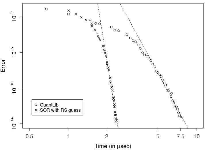
Example 1: Pricing error for plain vanilla options
- Market prices are given by the Black-Scholes-Merton model with
 .
.
- Normal-CLV process parameters are given by

Ten collocation points are used to define the mapping function and the time to maturity is one year. The diagram below shows the deviation of the implied volatility of the Normal-CLV price based on the PDE solution from the true value of 25%
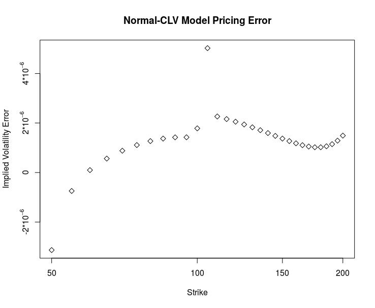
Even ten collocation points are already enough to obtain a very small pricing error. The advice in [2] to stretch the collocation grid has turned out to be very efficient if the number of collocation points gets larger.
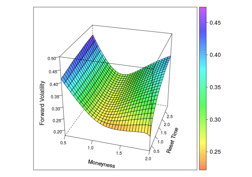
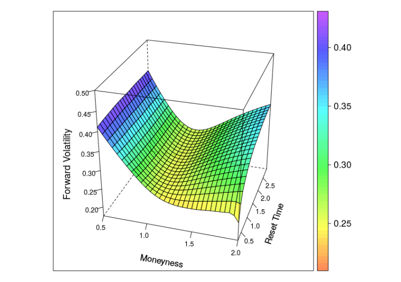
Example 2: Forward volatility skew
- Market prices are given by the Heston model with
 .
.
- Normal-CLV process parameters are given by

The diagram below shows the implied volatility of an forward starting European option with moneyness varying from 0.5 to 2 and maturity date six month after the reset date.

The shape of the forward volatility surface of the Normal-CLV model shares important similarities with the surfaces of the more complex Heston or Heston Stochastic Local Volatility (Heston-SLV) model with large mixing angles  . But by the very nature of the Normal-CLV model, the forward volatility does not depend on the values of
  or
or  , which limits the variety of different forward skew dynamics this model can create. CLV models with non-normal kernel processes will support a greater variety.
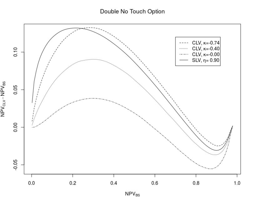
Example 3: Pricing of Double-no-Touch options
- Market prices are given by the Heston model with
 .
.
- Normal-CLV process parameters are given by different
 values and

Unsurprisingly the prices of 1Y Double-no-Touch options exhibit similar patterns with the Normal-CLV model and the Heston-SLV model as shown below in the “Moustache” graph. But the computational efforts using the Normal-CLV model are much smaller than the efforts for calibrating and solving the Heston-SLV model.
The QuantLib implementation of the Normal-CLV model is available as a pull request #117, the Rcpp based package Rclv contains the R interface to the QuantLib implementation and the demo code for all three examples.
[1] A. Grzelak, 2016, The CLV Framework – A Fresh Look at Efficient Pricing with Smile
[2] L.A. Grzelak, J.A.S. Witteveen, M.Suárez-Taboada, C.W. Oosterlee,
The Stochastic Collocation Monte Carlo Sampler: Highly efficient sampling from “expensive” distributions
[3] J-P. Berrut, L.N. Trefethen, Barycentric Lagrange interpolation, SIAM Review, 46(3):501–517, 2004.


 Diagrams are based on the test cases testHigerOrderBSOptionPricing and
 at time
  with strike
  and maturity
 in terms of the discount factor
  , the forward price
  and the moneyness
 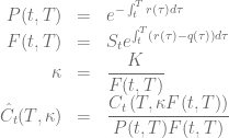 .
. is then given by
 .
. amd
amd  yields
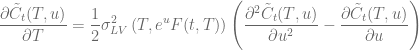
 are fulfilling the same equation, which can easily been shown by inserting the call-put parity into the equation above
 .
.
 w.r.t. time
  is given by


 The implementation is available
  of a piecewise constant time dependent Heston model
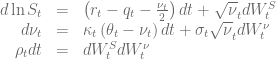
 time intervals
 ![[t_0=0, t_1], ... ,[t_{n-1}, t_n]](https://s0.wp.com/latex.php?latex=%5Bt_0%3D0%2C+t_1%5D%2C+...+%2C%5Bt_%7Bn-1%7D%2C+t_n%5D&bg=ffffff&fg=5e5e5e&s=0&c=20201002) and constant parameters within these intervals
and constant parameters within these intervals![\kappa_t = \kappa_j \wedge \theta_t = \theta_j \wedge \sigma_t=\sigma_j \wedge \rho_t=\rho_j \forall j\in [1, n] \wedge t\in [t_{j-1}, t_j]](https://s0.wp.com/latex.php?latex=%5Ckappa_t+%3D+%5Ckappa_j+%5Cwedge+%5Ctheta_t+%3D+%5Ctheta_j+%5Cwedge+%5Csigma_t%3D%5Csigma_j+%5Cwedge+%5Crho_t%3D%5Crho_j+%5Cforall+j%5Cin+%5B1%2C+n%5D+%5Cwedge+t%5Cin+%5Bt_%7Bj-1%7D%2C+t_j%5D&bg=ffffff&fg=5e5e5e&s=0&c=20201002)
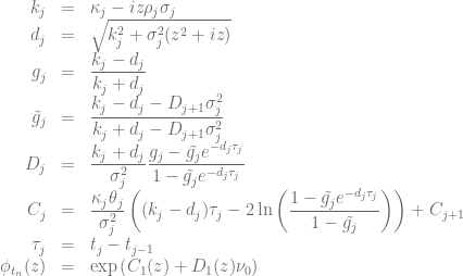
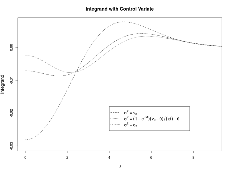
 in order to calculate the truncation point for the integral over the characteristic function when using the Andersen-Piterbarg approach with control variate [2]. A Mathematica script gives

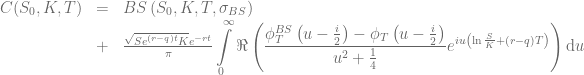
 of a vanilla call option with volatility
  and the characteristic function


 with
with  the second cumulant of
  [1].
[1].
 and maturity
  .
.
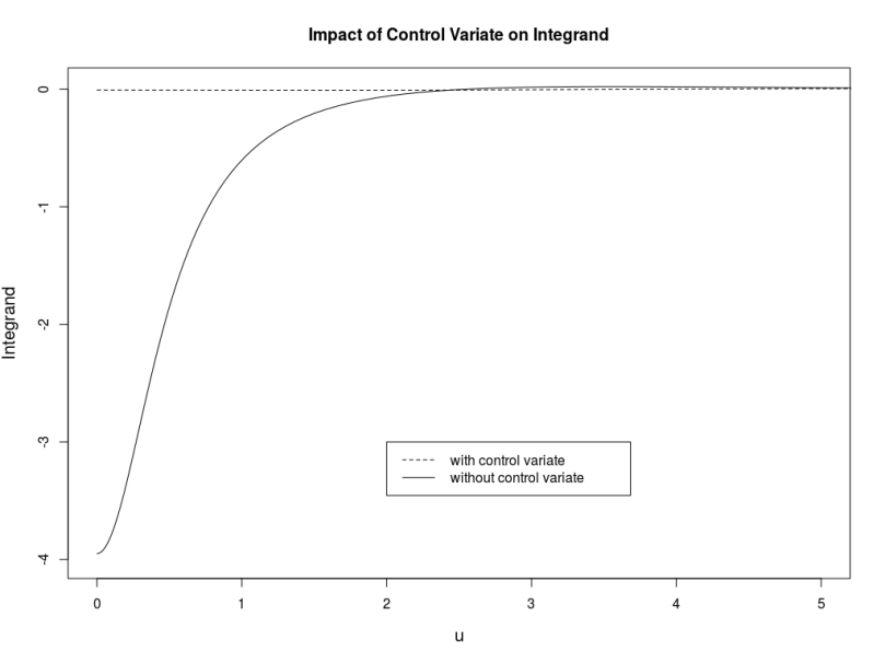
 such that the remaining part is smaller than a given threshold based on the following inequation
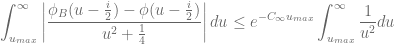


 given
given  is
is
 denotes the noncentral chi-squared distribution with
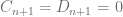
 and the minor diagonal
  . Again these vectors are defined by a recurrence relation [2]
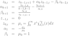
 of the noncentral chi-squared distribution can be calculated using Mathematica and exported as plain C code in order to be integrated into QuantLib.
 .
.