The Collocating Local Volatility Model

In a recent paper [1] Lech Grzelak has introduced his Collocating Local Volatility Model (CLV). This model utilises the so called collocation method [2] to map the cumulative distribution function of an arbitrary kernel process onto the true cumulative distribution function (CDF) extracted from option market quotes.

Starting point for the collocating local volatility model is the market implied CDF of an underlying $S_t$ at time $t_i$ :

$F_{S(t_i)}(x) = 1 + e^{r t_i}\frac{\partial V_{call}(t_0, t_i, K)}{\partial K}\mid_{K=x} = e^{r t_i}\frac{\partial V_{put}(t_0, t_i, K)}{\partial K}\mid_{K=x}$

The prices can also be given by another calibrated pricing model, e.g. the Heston model or the SABR model. To increase numerical stability it is best to use OTM calls and puts.

The dynamics of the spot process $S_t$ should be given by some stochastic process $X_t$ and a deterministic mapping function $g(t, x)$ such that

$S_t=g(t, X_t)$

The mapping function $g(t, x)$ ensures that the terminal distribution of $S_t$ given by the CLV model matches the market implied CDF. The model then reads

$\begin{array}{rcl} S_t &=& g(t,X_t) \nonumber \\ dX_t &=& \mu(X_t)dt + \sigma(X_t)dW_t\nonumber \end{array}$

The choice of the stochastic process $X_t$ does not influence the model prices of vanilla European options – they are given by the market implied terminal CDF – but influences the dynamics of the forward volatility skew generated by the model and therefore the prices of more exotic options. It is also preferable to choose an analytical trackable process $X_t$ to reduce the computational efforts.

The collocation methods outlined in [2] defines an efficient algorithm to approximate the mapping function $g(t, x)$ based on a set of collocation points $x_{i,j}=x_j(T_i)$ for a given set of maturities $T_i, i=1,...,m$ and $j=1,...,n$ interpolation points per maturity $T_i$ . Let $F_{S_{T_i}}(s)$ be the market implied CDF for a given expiry $T_i$ . Then we get

$\begin{array}{rcl} F_{X_{T_i}}\left(x_{i,j}\right) &=& F_{S_{T_i}}\left(g(T_i, x_{i,j})\right) = F_{S_{T_i}} \left(s_{i,j}\right) \nonumber \\ \Rightarrow s_{i,j}&=&F^{-1}_{S_{T_i}}\left(F_{X_{T_i}}(x_{i,j})\right) \nonumber \end{array}$

for the collocation points with $s_{i,j}=g(T_i, x_{i,j})$ .

The optimal collocation points are given by the abscissas of the Gaussian quadrature for the terminal distribution of $X_{T_i}$ . The simplest choice is a normally distribute kernel process $X_t$ like the Ornstein-Uhlenbeck process

$dX_t = \kappa(\theta-X_t)dt + \sigma dW_t$ .

The corresponding collocation points of the Normal-CLV model are then given by

$\begin{array}{rcl} x_j(t) &=& \mathbb{E}\left[X_t\right] + \sqrt{\mathbb{V}ar\left[X_t\right]} x_j^{\mathcal{N}(0,1)} \nonumber \\ &=& \theta + \left(X_0 - \theta)e^{-\kappa t}\right) + \sqrt{\frac{\sigma^2}{2\kappa}\left(1-e^{-2\kappa t}\right)} x_j^{\mathcal{N}(0,1)}, \ j=1,...,n\end{array}$

in which the collocation points $x_j^{\mathcal{N}(0,1)}$ of the standard normal distribution can be calculated by QuantLib’s Gauss-Hermite quadrature implementation

Array abscissas = std::sqrt(2)*GaussHermiteIntegration(n).x()

Lagrange polynomials [3] are an efficient interpolation scheme to interpolate the mapping function $g(t, x)$ between the collocation points

$g(t, X_t) = \sum_{j=1}^N s_j (t)\prod_{k=1, j\neq k}^N \frac{X(t)-x_j(t)}{x_k(t)-x_j(t)}$

Strictly speaking Lagrange polynomials do not preserve monotonicity and one could also use monotonic interpolation schemes supported by QuantLib’s spline interpolation routines. As outlined in [2] this method can also be used to approximate the inverse CDF of an “expensive” distributions.

Calibration of the Normal-CLV model to market prices is therefore pretty fast and straight forward as it takes the calibration of $g(t, x_t)$ .

Monte-Carlo pricing means simulating the trackable process $X_t$ and evaluate the Lagrange polynomial if the value of the spot process $S_t$ is needed. Pricing via partial differential equation involves the one dimensinal PDE

$\frac{\partial V}{\partial t} + \mu(x)\frac{\partial V}{\partial x} + \frac{1}{2}\sigma^2(x)\frac{\partial^2 V}{\partial x^2}-rV = 0$

with the terminal condition at maturity time $T$

$V(T, x_T) = \text{Payoff}\left(S_T=g(T,x_T)\right)$

For plain vanilla options the upper and lower boundary condition is

$\frac{\partial^2 V}{\partial x^2} = 0 \ \ \forall x\in\left\{x_{min},x_{max}\right\}$

Example 1: Pricing error for plain vanilla options

Market prices are given by the Black-Scholes-Merton model with

$S_0=100, r=0.1, q=0.04, \sigma=0.25$ .

Normal-CLV process parameters are given by

$\kappa=1.0, \theta=0.1,\sigma=0.5,x_0=0.1$

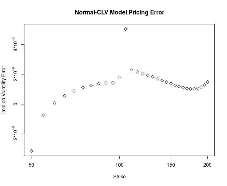
Ten collocation points are used to define the mapping function $g(t, x)$ and the time to maturity is one year. The diagram below shows the deviation of the implied volatility of the Normal-CLV price based on the PDE solution from the true value of 25%

clvpriceerror

Even ten collocation points are already enough to obtain a very small pricing error. The advice in [2] to stretch the collocation grid has turned out to be very efficient if the number of collocation points gets larger.

Example 2: Forward volatility skew

Market prices are given by the Heston model with

$S_0=100, r=0.1, q=0.05, \nu_o=0.09, \kappa=1.0, \theta=0.06, \sigma=0.4, \rho=-0.75$ .

Normal-CLV process parameters are given by

$\kappa=-0.075, \theta=0.05,\sigma=0.25,x_0=0.05$

The diagram below shows the implied volatility of an forward starting European option with moneyness varying from 0.5 to 2 and maturity date six month after the reset date.

hestonforward

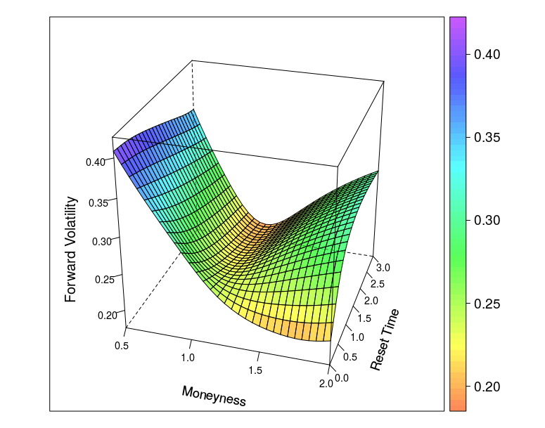
The shape of the forward volatility surface of the Normal-CLV model shares important similarities with the surfaces of the more complex Heston or Heston Stochastic Local Volatility (Heston-SLV) model with large mixing angles $\eta$ . But by the very nature of the Normal-CLV model, the forward volatility does not depend on the values of $\theta, \sigma$ or $x_0$ , which limits the variety of different forward skew dynamics this model can create. CLV models with non-normal kernel processes will support a greater variety.

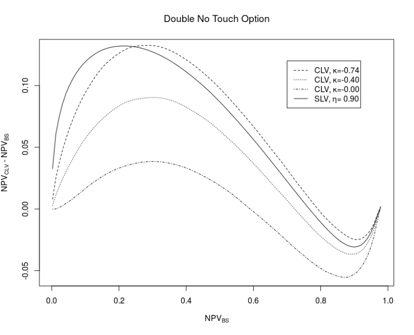
Example 3: Pricing of Double-no-Touch options

Market prices are given by the Heston model with

$S_0=100, r=0.02, q=0.01, \nu_o=0.09, \kappa=1.0, \theta=0.06, \sigma=0.8\rho=-0.8$ .

Normal-CLV process parameters are given by different $\kappa$ values and

$\theta=100,\sigma=0.15,x_0=100.0$

Unsurprisingly the prices of 1Y Double-no-Touch options exhibit similar patterns with the Normal-CLV model and the Heston-SLV model as shown below in the “Moustache” graph. But the computational efforts using the Normal-CLV model are much smaller than the efforts for calibrating and solving the Heston-SLV model.

The QuantLib implementation of the Normal-CLV model is available as a pull request #117, the Rcpp based package Rclv contains the R interface to the QuantLib implementation and the demo code for all three examples.

[1] A. Grzelak, 2016, The CLV Framework – A Fresh Look at Efficient Pricing with Smile

[2] L.A. Grzelak, J.A.S. Witteveen, M.Suárez-Taboada, C.W. Oosterlee,
The Stochastic Collocation Monte Carlo Sampler: Highly efficient sampling from “expensive” distributions

[3] J-P. Berrut, L.N. Trefethen, Barycentric Lagrange interpolation, SIAM Review, 46(3):501–517, 2004.

HPC-QuantLib

The Collocating Local Volatility Model

Leave a comment Cancel reply

Share this:

Related

Leave a comment Cancel reply